Assignment 2
Deconstruct, Reconstruct Web Report
Su Myat Noe Yee (s3913797)
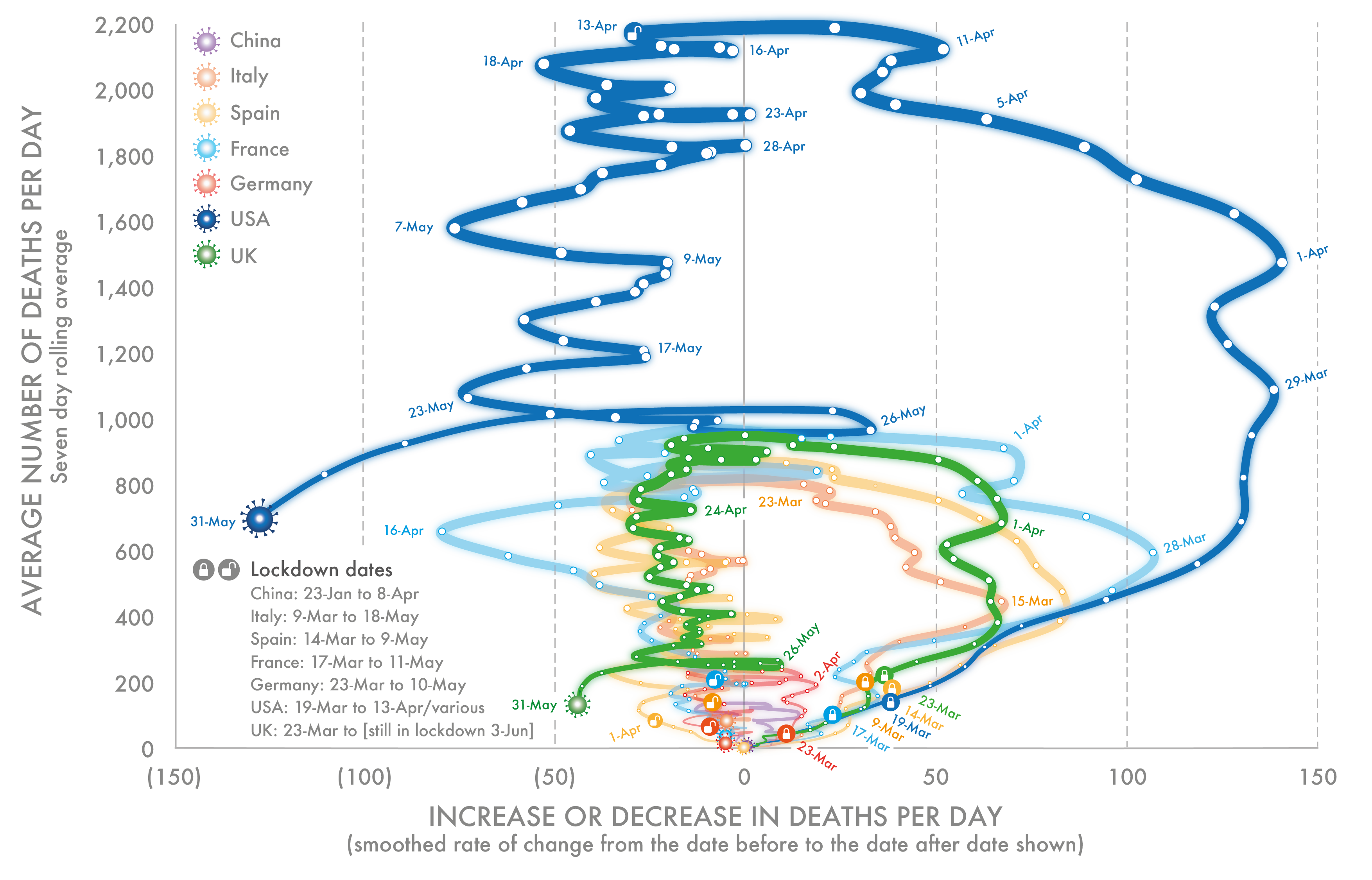
This report will include 3 parts: (1) Original data visualization (2) Code to improve the issues in original data visulisation and (3) Reconstruction of original data visulisation. The visulisation shows the mortality in 7 countries: USA, France, Spain, Italy, UK, China and Germany, attributed to Covid 19 during period 23 January 2020 to 31 May 2020. Here, the average number of deaths per day is calculated as seven day rolling average whereas increase/ decrease in deaths per day is obtained from smooth rate of change from the date before to the date after the date shown.
Click the Original, Code and Reconstruction tabs to read about the issues and how they were fixed.
Original

Objective
The objective of this data visualization is to show the mortality in seven countries USA, France, Spain, Italy, UK, China and Germany attributed to Covid 19 using two factors (1) Average number of deaths per day and (2) Increase/ Decrease in deaths per day during period 23 January 2020 to 31 May 2020.
As conventional graphs focus to show the number of deaths reported each day for various countries, the audience is still left trying to discern the extent to which the rise from one day to the next is larger or slower. So, these graphs is targeted to audience who are willing to know the rate of death changes per day along with average number of deaths per day.
The visualization chosen had the following three main issues:
- Perceptual and color issue - The color usage here might cause issue color-blind people. If audience have tritanomaly, blue and green will look the same.Even though there is a legend, the country name is shown with color. So, they will not know which line is USA and which is UK. To solve those issue, a label or description of each country will be added to each line/ graph. The issue can also be solved by avoid using colors which can cause problem to color-blind people.
- Visual bombardment (Deception Method) - In this graph, the audience will get confuse what the visualization want to show. All the variables: time, countries, rate of death of change and average number of deaths, lockdown dates are shown together in one visualization (without faceting) which lead to audience’s confusion. It’s hard to see China and Germany data as the others countries death rate are very high compared to those two countries. Using birght and thick line for USA makes all the focus go to only that country which is leading to deception. Showing deaths and changes of death of each country in separate graphs rather than combing all the data: deaths and changes of deaths of all countries in one graph in more efficient, effective and clearer for the audience. They will be able to see information more clearly such as which date has highest deaths or lowest deaths.
- Date Integrity - In the visualization, the source of the data is not mentioned as well as the targeted audience for particular visualization. Moreover, the data usage in the visualization is not align with what describe in the introduction of the blog. For example, in visualization, y-axis label is “Average number of deaths per day (seven day rolling average) whereas in the introduction of the blog, it’s said”Average number of death is the simple average of the number that occurred the day before and the day after.” One of the information needs to be changed in order to fix that issue.
Reference
- Dorling, D. (2020). Slowdown Covid 19. https://www.dannydorling.org/books/SLOWDOWN/Covid19.html
- Dorling, D. (2020). Mortality in seven countries attributed to Covid-19 (23 January to 31 May 2020). https://www.dannydorling.org/books/SLOWDOWN/Images/Cv19Fatalities3Jun2020-01.png 8 Center for Systems Science and Engineering at Johns Hopkins University. (n.d.). COVID-19 Data Repository. https://github.com/CSSEGISandData/COVID19/blob/master/csse_covid_19_data/csse_covid_19_time_series/time_series_covid19_deaths_global.csv
- GeeksForGeeks. (2021, May 21). ggplot2-Title and Subtitle with different size and color in R. https://www.geeksforgeeks.org/ggplot2-title-and-subtitle-with-different-size-and-color-in-r/#:
- Zach. (2020, Oct 2020). How to change legend size in ggplot2 with examples. Statology. https://www.statology.org/ggplot2-legend-size/
Code
The following code was used to fix the issues identified in the original.
#Installing necessary packages
library(ggplot2)
library(magrittr)
library(dplyr)
library(ggpubr)
library(readxl)
library(tidyr)
library(ggh4x)

#Setting up working directory and loading data file into working environment
setwd("~/Desktop/2nd Sem/Visualisation/Assignment 2")
data <- read_excel("~/Desktop/2nd Sem/Visualisation/Assignment 2/Visualisation.xlsx")

#Tidying and reconstructing the dataset
unitedata <- unite(data, col='Countryanddate', c('Country', 'Date'), sep='@')
tidydata <- gather(unitedata, key='Type', value = 'Value', 2:3 )
finaldata <- tidydata %>% separate(Countryanddate, into = c("Country","Date"), sep='@')
finaldata$Date <- as.Date(finaldata$Date)

#Deconstruct and Reconstructing
datavis <- ggplot(finaldata, aes(Date, Value, group = 1)) +
  geom_line(aes(color = Country), size=1.4)+
  geom_point(color="white", size=0.05) +
  scale_x_date(date_breaks = "1 months", date_labels = "%e-%b") +
  labs(title = "Mortality in Seven Countries attributed to Covid-19",
       subtitle = "(From 23 January to 31 May 2020.)",
       y = "",
       x = "Date",
       caption = "Data Source: COVID-19 Data Repository by CSSE at Johns Hopkins University") +
  facet_grid(Country~Type, switch = "y", scale= "free_y") +
  theme(
  panel.background = element_rect(fill = "#BFD5E3", colour = "#6D9EC1", size = 2.5, linetype = "solid"),
  panel.grid.minor = element_line(size = 0.15, linetype = 'solid', colour = "white"),
  panel.grid.major = element_line(size = 0.3, linetype = 'solid', colour = "white"),
  plot.background = element_rect(fill = "#BFD5E3"),
  strip.background = element_rect(fill="#6D9EC1"), #Changing color of facet label background color
  strip.text = element_text(color = "white", size = 14), #Changing text size and color of facet grid label
  plot.title = element_text(size = 16), #Changing text size of visualization title
  plot.subtitle = element_text (size=12), #Changing text size of visualization subtitle
  plot.caption = element_text(size = 12), #Changing text size of visualization caption
  legend.position = "bottom", #Changing legend location to bottom
  legend.title = element_text(size=10), #Changing legend title size
  legend.text = element_text(size=9) #Changing legend text size
  ) +
  scale_color_discrete(name = "Lockdown Period",
                       labels=c("China : 23-Jan to 8-Apr",
                                "France : 17-Mar to 11-May",
                                "Germany : 23-Mar to 10-May ",
                                "Italy : 9-Mar to 18-May",
                                "Spain : 14-Mar to 9-May",
                                "USA : 19-Mar to 13-Apr",
                                "UK : 23-Mar to 3-Jun"))
Data Reference
- Dorling, D. (2020). Slowdown Covid 19. https://www.dannydorling.org/books/SLOWDOWN/Covid19.html
- Dorling, D. (2020). Mortality in seven countries attributed to Covid-19 (23 January to 31 May 2020). https://www.dannydorling.org/books/SLOWDOWN/Images/Cv19Fatalities3Jun2020-01.png 8 Center for Systems Science and Engineering at Johns Hopkins University. (n.d.). COVID-19 Data Repository. https://github.com/CSSEGISandData/COVID19/blob/master/csse_covid_19_data/csse_covid_19_time_series/time_series_covid19_deaths_global.csv
- GeeksForGeeks. (2021, May 21). ggplot2-Title and Subtitle with different size and color in R. https://www.geeksforgeeks.org/ggplot2-title-and-subtitle-with-different-size-and-color-in-r/#:
- Zach. (2020, Oct 2020). How to change legend size in ggplot2 with examples. Statology. https://www.statology.org/ggplot2-legend-size/
Reconstruction
The following plot fixes the main issues in the original.
