ANLY 512 - Problem Set #2
Intro to Data Visualizations
Bingqing Li
2022-09-18
Directions
In this chapter we discussed wy well-designed data graphics are important and we described a taxonomy for understanding their composition.
The objective of this assignment is for you to understand what characteristics you can use to develop a great data graphic.
Each question is worth 5 points.
To submit this homework you will create the document in Rstudio, using the knitr package (button included in Rstudio) and then submit the document to your Rpubs account. Once uploaded you will submit the link to that document on Canvas. Please make sure that this link is hyper linked and that I can see the visualization and the code required to create it.
Question #1
Answer the following questions for this graphic Relationship between ages and psychosocial maturity
- Identify the visual cues, coordinate system, and scale(s)
- How many variables are depicted in the graph? Explicitly link each variable to a visual cue that you listed above.
- Critique this data graphic using the taxonomy described in the lecture.
This plot uses position on both vertical and horizontal scales. The visual cue of color represents different categories. The green one is about Menarche while the pink one is about Psychosocial Maturation. The visual cue of length represents the Age span of when a female meets the category mentioned above on the vertical axis with a linear scale. It also adds labels next to the rectangular and uses matched colors. The ordinal variable of time is arrayed on the horizontal axis. The lines between different time segments is the visual cue of directions, which is used to indicate the progression of human evolvement. The coordinate system is Cartesian. Context is provided by the axis labels and annotations like the era of the time and “Mismatch” conclusion.
Question #2
Answer the following questions for this graphic World’s top 10 best selling cigarette brands 2004-2007
- Identify the visual cues, coordinate system, and scale(s)
- How many variables are depicted in the graph? Explicitly link each variable to a visual cue that you listed above.
- Critique this data graphic using the taxonomy described in the lecture.
This plot uses the visual cue of length to represent the Cigarette sales on the horizontal axis with a linear scale. It also uses the visual cue of color to represent different cigarette brands. The categorical variable of the top brands is arrayed on the vertical axis. The coordinate system is Cartesian. Context is provided by the axis labels and title.
Question #3
Find two data graphics published in a newspaper or on the internet in the last two years.
- Identify a graphical display that you find compelling. What aspects of the display work well, and how do these relate to the principles that we have just gone over in lecture. Include a screenshot of the display along with your solution (Hint:use the following in a code chunk: knitr::include_graphics(“your_graphic”).
knitr::include_graphics("ChainnessUA.png")
I find this map compelling, because I can easily identify that high chainness cities are prevalent in the Midwestern and the Southeastern United States whereas low chainness was more associated with East and West Coast cities, using the visual cue of color. The redder the city, the higher the chainness. The bluer the city, the lower the chainness. It uses a geographic map with major cities labels, so that viewers can easily distinguish the difference between chain restaurants and independent ones in terms of locations. Context is provided by legends, a map scale and a title.
- Identify a graphical display that you find less compelling. What aspects of the display don’t work well? Are there ways that the display might be improved? Include a screenshot of the display along with your solution (Hint:use the following in a code chunk: knitr::include_graphics(“your_graphic”).
knitr::include_graphics("where-the-memes-came-from.png")
I find this graph less compelling, because 1. some colors of the social media are mixed with the dark background. My suggestion is to use more vivid colors to pop up the top social media like TikTok and Twitter, or simply change the background color to white. 2. It’s difficult to read the graph and understand which line is which social media from the legend aside. When it comes to multiple categories in a legend, my suggestion is either put a label next to the end of each line, or order the legend the same way as the end of the line is ordered, to reduce the back and forth between the lines and the legend when people read the graph. 3. I don’t see a reason to use double-digit decimals on the Y-axis, which makes the chart messier than it should’ve been.
Question #4
Briefly (one paragraph) critique the designer’s choices. Would you have made different choices? Why or why not? Note: Link contains a collection of many data graphics, and I don’t expect (or want) you to write a full report on each individual graphic. But each collection shares some common stylistic elements. You should comment on a few things that you notice about the design of the collection.
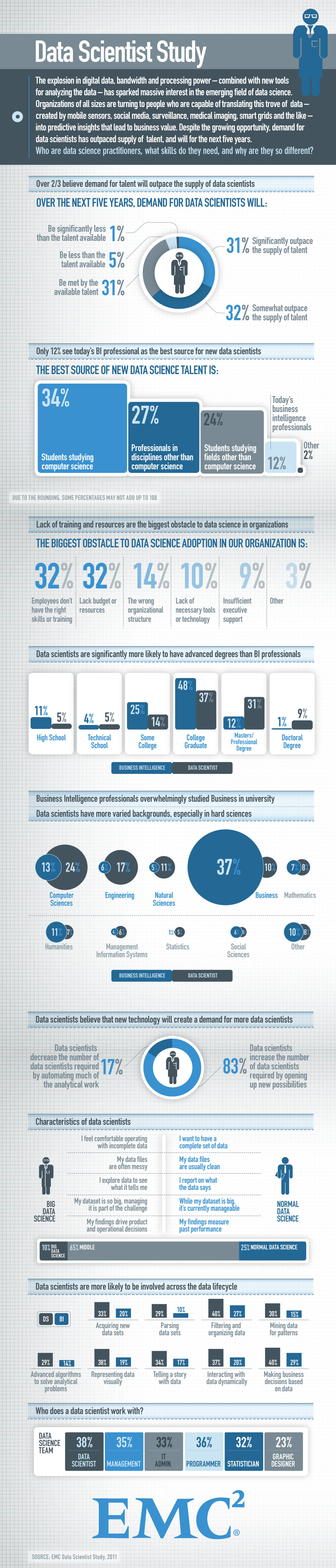
Answer:
I really like the infographics overall. It has many comparisons for this study and uses appropriate as well as versatile charts to show its conclusion. It uses donut chart to show survey results - what percentage of people believe this and that. It uses bar chart and side by side bar chart when it comes to categorical data like data scientists’ education and data lifecycle. However, there are 2 things that I’ll do differently. 1. I’ll match the shade of the color with the numbers. For example, navy blue will be used for the highest percentage rather than the 2nd highest one in the donut charts. 2. For the last graph - who data scientists work with, I’ll put different parties in descending order of the %time they work with.
Question #5
Briefly (one paragraph) critique the designer’s choices. Would you have made different choices? Why or why not? Note: Link contains a collection of many data graphics, and I don’t expect (or want) you to write a full report on each individual graphic. But each collection shares some common stylistic elements. You should comment on a few things that you notice about the design of the collection.
Charts that explain food in America
Answer:
This collection shows us that there are many ways to visualize your data even if using just a map. You could use dots and 2 colors to represent a location’s farm increase/decrease. You could fill the map with sequential or divergent color palettes to show agricultural products sold in different areas. You can also associate brand logos with states. Furthermore, you could add town information in addition to the state-wise info like the map “Where you can drink on the street”. My favorite of this collection of graphs is No.37 where labels of popular products are added to the map. Given context like that, the graph is more readable. The visual cue of color indicates states where hot or ice beverages are more popular. Overall, the map is concise but straightforward. What I found confusing, however, in this collection is No. 11, the pie chart. It took me some time to understand what the degree of each slide means. My suggestion would be either adding the % under the $ or change it to a horizontal bar chart.