Becoming an AnimatoR

# Becoming an AnimatoR
## Applications in `ggplot`, `gganimate`, and more!

### Brady Rippon
### WCM Biostatistics Computing Club
### August 02, 2022

---

# Grammar of Graphics

---

background-image: url(https://raw.githubusercontent.com/bradyrippon/Images_WCM/main/drake.png)
background-size: 550px
background-position: 50% 70%

# Using `ggplot` v. base R?

---

# Using `ggplot` v. base R?

- Customize your **themes** for any style you like!

<code class ='r hljs remark-code'>ggplot(iris, aes(x = Sepal.Length, &nbsp;&nbsp;&nbsp;&nbsp;&nbsp;&nbsp;&nbsp;&nbsp;&nbsp;&nbsp;&nbsp;&nbsp;&nbsp;&nbsp;&nbsp;&nbsp;&nbsp;y = Sepal.Width)) + &nbsp;&nbsp;geom_jitter(alpha = 0.6) + &nbsp;&nbsp;facet_grid(. ~ Species) + &nbsp;&nbsp;stat_smooth(method = "lm", &nbsp;&nbsp;&nbsp;&nbsp;&nbsp;&nbsp;&nbsp;&nbsp;&nbsp;&nbsp;&nbsp;&nbsp;&nbsp;&nbsp;se = F, col = "red") + &nbsp;&nbsp;scale_y_continuous("Sepal Width (cm)", &nbsp;&nbsp;&nbsp;&nbsp;&nbsp;&nbsp;&nbsp;&nbsp;&nbsp;&nbsp;&nbsp;&nbsp;&nbsp;&nbsp;&nbsp;&nbsp;&nbsp;&nbsp;&nbsp;&nbsp;&nbsp;limits = c(2, 5), &nbsp;&nbsp;&nbsp;&nbsp;&nbsp;&nbsp;&nbsp;&nbsp;&nbsp;&nbsp;&nbsp;&nbsp;&nbsp;&nbsp;&nbsp;&nbsp;&nbsp;&nbsp;&nbsp;&nbsp;&nbsp;expand = c(0, 0)) + &nbsp;&nbsp;scale_x_continuous("Sepal Length (cm)", &nbsp;&nbsp;&nbsp;&nbsp;&nbsp;&nbsp;&nbsp;&nbsp;&nbsp;&nbsp;&nbsp;&nbsp;&nbsp;&nbsp;&nbsp;&nbsp;&nbsp;&nbsp;&nbsp;&nbsp;&nbsp;limits = c(4, 8), &nbsp;&nbsp;&nbsp;&nbsp;&nbsp;&nbsp;&nbsp;&nbsp;&nbsp;&nbsp;&nbsp;&nbsp;&nbsp;&nbsp;&nbsp;&nbsp;&nbsp;&nbsp;&nbsp;&nbsp;&nbsp;expand = c(0, 0)) + &nbsp;&nbsp;coord_equal() + &nbsp;&nbsp;theme()</code>

]

![](https://raw.githubusercontent.com/bradyrippon/Images_WCM/main/layers2.png)
![](https://raw.githubusercontent.com/bradyrippon/Images_WCM/main/exampleGG.png)

]

---

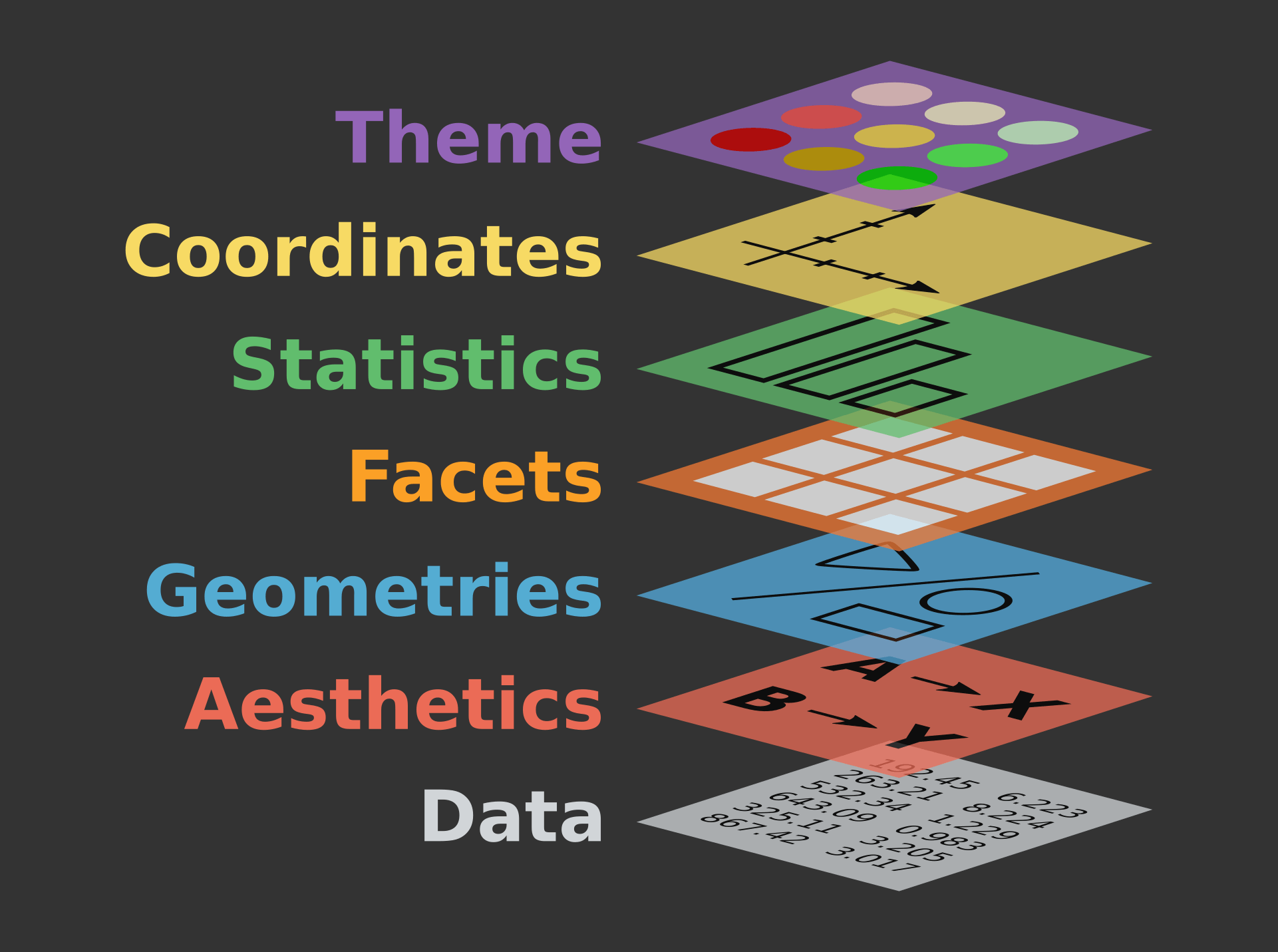# Explore different `ggplot` extensions!

```r
library(ggridges)
plot_a <- ggplot(iris) +
* geom_density_ridges(aes(fill = Species)) + # custom geometric layer
 (...) # additional layers
 
library(ggalt)
iris_setosa <- iris %>% filter(Species == "setosa")
plot_b <- ggplot(iris) +
* geom_encircle(data = iris_setosa) + # custom geometric layer
 (...) # additional layers

library(ggforce)
plot_c <- ggplot(iris) +
* facet_zoom(x = Species == "versicolor") + # custom facet layer
 (...) # additional layers

library(ggpubr) # also includes many plotting extensions
ggarrange(plot_a, plot_b, plot_c, ncol = 3, nrow = 1, 
          common.legend = TRUE, legend = "bottom", labels = "AUTO")
```

---

# Explore different `ggplot` extensions!

![Image description](https://raw.githubusercontent.com/bradyrippon/Images_WCM/main/GGgallery.png)

---

background-image: url(https://raw.githubusercontent.com/bradyrippon/Images_WCM/main/passionCat.png)
background-size: 500px
background-position: 80% 85%

# `ggplot` Resources

Public materials and tutorials:

- Package documentation from [tidyverse website](https://ggplot2.tidyverse.org/)

- Browse the [R graph gallery](https://r-graph-gallery.com/) for more extensions and figure examples

WCM Computing Club materials:

- [The Beauty of `ggplot2`](https://wcm-computing-club.github.io/file_resources/Lee_R_ggplot2.html) by Dr. Jihui Lee

- [Visualization in R](https://wcm-computing-club.github.io/file_slides/2019/201904_Cooley_Visualization_in_R.html#introduction) by Vicky Cooley

---

# The Animation Layer

---

# Add a custom animation layer

The **gganimate** package provides a new range of grammar classes which can be added to the `ggplot` plot object

- **transition*_()** defines how long the data should be spread out and how long it relates to itself across time

- **shadow*_()** defines how the data from other points in time should be presented in the given point in time

- **enter*_()** / **exit*_()** defines how new data should appear and how old data should disappear during the course of the animation

- **ease_aes()** defines how different aesthetics should be eased during transitions 
]

---

# The **transition*_()** function

This function could take the following form:

- **transition_states()**: Transition between several distinct stages of the data

- **transition_reveal()**: Reveal data along a given dimension

- **transition_events()**: Transition individual events in and out

- **transition_filter()**: Transition between different filters

- **transition_layers()**: Build up a plot, layer by layer

- **transition_components()**: Transition individual components through their own lifecycle

- **transition_manual()**: Create an animation by specifying the frame membership directly

- **transition_null()**: Keep all data constant across the animation
]

---

# Example: **transition_states()**:

```r
ggplot(iris, aes(Sepal.Width, Petal.Width)) +
  geom_point() +
* transition_states(Species, transition_length = 3, state_length = 1)
```

.center[
<img src="https://raw.githubusercontent.com/bradyrippon/Images_WCM/main/t_s.gif" width="500px" />
]

---

# The **transition*_()** function

This function could take the following form:

- **transition_time()**: Transition through distinct states in time

- **transition_events()**: Transition individual events in and out

- **transition_filter()**: Transition between different filters

- **transition_layers()**: Build up a plot, layer by layer

- **transition_components()**: Transition individual components through their own lifecycle

- **transition_manual()**: Create an animation by specifying the frame membership directly

- **transition_null()**: Keep all data constant across the animation
]

---

# Example: **transition_time()**:

```r
ggplot(airquality, aes(Day, Temp)) +
  geom_point(aes(colour = factor(Month))) +
* transition_time(Day) # coerces raw values into the closest frame
```

.center[
<img src="https://raw.githubusercontent.com/bradyrippon/Images_WCM/main/t_t.gif" width="800px" />
]

---

# The **transition*_()** function

This function could take the following form:

- **transition_time()**: Transition through distinct states in time
]

- **transition_reveal()**: Reveal data along a given dimension

- **transition_filter()**: Transition between different filters

- **transition_layers()**: Build up a plot, layer by layer

- **transition_components()**: Transition individual components through their own lifecycle

- **transition_manual()**: Create an animation by specifying the frame membership directly

- **transition_null()**: Keep all data constant across the animation
]

---

# Example: **transition_reveal()**:

```r
ggplot(airquality, aes(Day, Temp, group = Month)) +
  geom_line(aes(colour = factor(Month))) +
* transition_reveal(Day) # calculates intermediary values at exact positions
```

.center[
<img src="https://raw.githubusercontent.com/bradyrippon/Images_WCM/main/t_r.gif" width="800px" />
]

---

# The **transition*_()** function

This function could take the following form:

- **transition_time()**: Transition through distinct states in time

- **transition_reveal()**: Reveal data along a given dimension
]

- **transition_events()**: Transition individual events in and out

- **transition_layers()**: Build up a plot, layer by layer

- **transition_components()**: Transition individual components through their own lifecycle

- **transition_manual()**: Create an animation by specifying the frame membership directly

- **transition_null()**: Keep all data constant across the animation
]

---

# Example: **transition_events()**:

```r
# create sample data
set.seed(1)

data <- data.frame(
 x = 1:10,
 y = runif(10),
 begin = runif(10, 1, 100),
 length = runif(10, 5, 20),
 enter = runif(10, 5, 10),
 exit = runif(10, 5, 10)
)

ggplot(data, aes(x, y)) +
  geom_col() +
* transition_events(start = begin,
*                   end = begin + length,
*                   enter_length = enter,
*                   exit_length = exit)
```
]

.pull-right[
.center[
<img src="https://raw.githubusercontent.com/bradyrippon/Images_WCM/main/t_e.gif" width="500px" />
]
]
---

# The **transition*_()** function

This function could take the following form:

- **transition_time()**: Transition through distinct states in time

- **transition_reveal()**: Reveal data along a given dimension

- **transition_events()**: Transition individual events in and out
]

- **transition_filter()**: Transition between different filters

- **transition_components()**: Transition individual components through their own lifecycle

- **transition_manual()**: Create an animation by specifying the frame membership directly

- **transition_null()**: Keep all data constant across the animation
]

---

# Example: **transition_filter()**:

```r
ggplot(iris, aes(Petal.Width, Petal.Length, 
                 colour = Species)) +
  geom_point() +
* transition_filter(
*   transition_length = 3,
*   filter_length = 1,
*   Setosa = Species == 'setosa',
*   Long = Petal.Length > 4,
*   Wide = Petal.Width > 2
* ) +
  theme(legend.position = "bottom")

# transition_filter(keep = T)
# Will keep previous data

# Can also control 
# enter() / exit() parameters
```
]

.pull-right[
.center[
<img src="https://raw.githubusercontent.com/bradyrippon/Images_WCM/main/t_f.gif" width="500px" />
]
]

---

# The **transition*_()** function

This function could take the following form:

- **transition_time()**: Transition through distinct states in time

- **transition_reveal()**: Reveal data along a given dimension

- **transition_events()**: Transition individual events in and out

- **transition_filter()**: Transition between different filters
]

- **transition_layers()**: Build up a plot, layer by layer

.secondary[
- **transition_components()**: Transition individual components through their own lifecycle

- **transition_manual()**: Create an animation by specifying the frame membership directly

- **transition_null()**: Keep all data constant across the animation
]

---

# Example: **transition_layers()**:

```r
ggplot(mtcars, aes(mpg, disp)) +
  geom_point() +
  geom_smooth(colour = 'grey', se = FALSE) +
  geom_smooth(aes(colour = factor(gear))) +
* transition_layers(layer_length = 1,
*               transition_length = 2,
*               from_blank = FALSE,
*               keep_layers = c(Inf, 0, 0)) +
  theme(legend.position = "bottom")

# Treats each plotting layer
# like a "state"
```
]

.pull-right[
.center[
<img src="https://raw.githubusercontent.com/bradyrippon/Images_WCM/main/t_l.gif" width="500px" />
]
]

---

# The **transition*_()** function

This function could take the following form:

- **transition_time()**: Transition through distinct states in time

- **transition_reveal()**: Reveal data along a given dimension

- **transition_events()**: Transition individual events in and out

- **transition_filter()**: Transition between different filters

- **transition_layers()**: Build up a plot, layer by layer
]

- **transition_components()**: Transition individual components through their own lifecycle

.secondary[
- **transition_manual()**: Create an animation by specifying the frame membership directly

- **transition_null()**: Keep all data constant across the animation
]

---

# Example: **transition_components()**:

```r
# create sample data
set.seed(1)

data <- data.frame(
 x = runif(10),
 y = runif(10),
 size = sample(1:3, 10, TRUE),
 time = c(1, 4, 6, 7, 9, 6, 7, 8, 9, 10),
 id = rep(1:2, each = 5)
)

ggplot(data, aes(x, y, group = id, 
                 size = size)) +
  geom_point() +
* transition_components(time,
*                       range = c(4, 8)) +
  theme(legend.position = "bottom")

# No common "state" and "transition"
```
]

.pull-right[
.center[
<img src="https://raw.githubusercontent.com/bradyrippon/Images_WCM/main/t_c.gif" width="500px" />
]
]

---

# The **transition*_()** function

This function could take the following form:

- **transition_time()**: Transition through distinct states in time

- **transition_reveal()**: Reveal data along a given dimension

- **transition_events()**: Transition individual events in and out

- **transition_filter()**: Transition between different filters

- **transition_layers()**: Build up a plot, layer by layer

- **transition_components()**: Transition individual components through their own lifecycle
]

- **transition_manual()**: Create an animation by specifying the frame membership directly

---

# Example: **transition_manual()**:

- Use with caution! Can often have rendering issues with frame count. The plot below is generated with **transition_states()**

```r
ggplot(mtcars, aes(gear, mpg)) +
  geom_boxplot() +
* transition_manual(gear) # no "tweening"; creates a 3-frame animation
```

.center[
<img src="https://raw.githubusercontent.com/bradyrippon/Images_WCM/main/t_m.gif" width="500px" />
]

---

# The **transition*_()** function

This function could take the following form:

- **transition_time()**: Transition through distinct states in time

- **transition_reveal()**: Reveal data along a given dimension

- **transition_events()**: Transition individual events in and out

- **transition_filter()**: Transition between different filters

- **transition_layers()**: Build up a plot, layer by layer

- **transition_components()**: Transition individual components through their own lifecycle

- **transition_manual()**: Create an animation by specifying the frame membership directly
]

- **transition_null()**: Keep all data constant across the animation

---

# Add a custom animation layer

The **gganimate** package provides a new range of grammar classes which can be added to the `ggplot` plot object

.secondary[
- **transition*_()** defines how long the data should be spread out and how long it relates to itself across time
]

- **view*_()** defines how the position scales should change along the animation

.secondary[
- **shadow*_()** defines how the data from other points in time should be presented in the given point in time

- **enter*_()** / **exit*_()** defines how new data should appear and how old data should disappear during the course of the animation

- **ease_aes()** defines how different aesthetics should be eased during transitions 
]

---

# **view*_(): view_follow()**

```r
transition_states_plot +
* view_follow(fixed_x = TRUE) # OR: view_follow(fixed_x = c(4, NA), y(...))
```

.pull-left[
.center[
<img src="https://raw.githubusercontent.com/bradyrippon/Images_WCM/main/t_s2.gif" width="400px" />
]
]

.pull-right[
.center[
<img src="https://raw.githubusercontent.com/bradyrippon/Images_WCM/main/v_f.gif" width="400px" />
]
]
---

# **view*_(): view_step()**

- Also explore **view_step_manual()**!

```r
transition_states_plot +
* view_step(pause_length = 3, step_length = 1,
*           nsteps = 3) # view_follow() with less static elements
```

.pull-left[
.center[
<img src="https://raw.githubusercontent.com/bradyrippon/Images_WCM/main/t_s2.gif" width="400px" />
]
]

.pull-right[
.center[
<img src="https://raw.githubusercontent.com/bradyrippon/Images_WCM/main/v_s.gif" width="400px" />
]
]

---

# **view*_(): view_zoom()**

- Also explore **view_zoom_manual()**!

```r
transition_states_plot +
* view_zoom(pause_length = 1, step_length = 2,
*           nsteps = 3, pan_zoom = -2) # view_step() with smooth zoom and pan
```

.pull-left[
.center[
<img src="https://raw.githubusercontent.com/bradyrippon/Images_WCM/main/t_s2.gif" width="400px" />
]
]

.pull-right[
.center[
<img src="https://raw.githubusercontent.com/bradyrippon/Images_WCM/main/v_z.gif" width="400px" />
]
]

---

# Add a custom animation layer

The **gganimate** package provides a new range of grammar classes which can be added to the `ggplot` plot object

.secondary[
- **transition*_()** defines how long the data should be spread out and how long it relates to itself across time

- **view*_()** defines how the position scales should change along the animation
]

- **shadow*_()** defines how the data from other points in time should be presented in the given point in time

.secondary[
- **enter*_()** / **exit*_()** defines how new data should appear and how old data should disappear during the course of the animation

- **ease_aes()** defines how different aesthetics should be eased during transitions 
]

---

# **shadow*_(): shadow_wake()**

```r
transition_states_plot +
* shadow_wake(wake_length = 0.05, colour = 'grey90') # (... size, alpha, etc.)
```

.pull-left[
.center[
<img src="https://raw.githubusercontent.com/bradyrippon/Images_WCM/main/t_s2.gif" width="400px" />
]
]

.pull-right[
.center[
<img src="https://raw.githubusercontent.com/bradyrippon/Images_WCM/main/s_w.gif" width="400px" />
]
]

---

# **shadow*_(): shadow_trail()**

```r
transition_time_plot +
* shadow_trail(0.02) # will keep every n-th frame, (... max_frames = N)
```

.pull-left[
.center[
<img src="https://raw.githubusercontent.com/bradyrippon/Images_WCM/main/t_t2.gif" width="400px" />
]
]

.pull-right[
.center[
<img src="https://raw.githubusercontent.com/bradyrippon/Images_WCM/main/s_t.gif" width="400px" />
]
]

---

# **shadow*_(): shadow_mark()**

```r
ggplot(airquality, aes(Day, Temp)) +
  geom_line() + transition_time(Month) +
* shadow_mark(color = "grey", size = 0.75) # (... past = T, future = F)
```

.pull-left[
.center[
<img src="https://raw.githubusercontent.com/bradyrippon/Images_WCM/main/s_m1.gif" width="400px" />
]
]

.pull-right[
.center[
<img src="https://raw.githubusercontent.com/bradyrippon/Images_WCM/main/s_m2.gif" width="400px" />
]
]

---

# Add a custom animation layer

The **gganimate** package provides a new range of grammar classes which can be added to the `ggplot` plot object

.secondary[
- **transition*_()** defines how long the data should be spread out and how long it relates to itself across time

- **view*_()** defines how the position scales should change along the animation

- **shadow*_()** defines how the data from other points in time should be presented in the given point in time
]

- **enter*_()** / **exit*_()** defines how new data should appear and how old data should disappear during the course of the animation

---

# **enter() / exit()**

```r
transition_manual_plot +
* enter_fade() + exit_fly(x_loc = 7, y_loc = 40)
```

.pull-left[
.center[
<img src="https://raw.githubusercontent.com/bradyrippon/Images_WCM/main/t_m2.gif" width="400px" />
]
]

.pull-right[
.center[
<img src="https://raw.githubusercontent.com/bradyrippon/Images_WCM/main/t_m2_ee.gif" width="400px" />
]
]

---

# Add a custom animation layer

The **gganimate** package provides a new range of grammar classes which can be added to the `ggplot` plot object

.secondary[
- **transition*_()** defines how long the data should be spread out and how long it relates to itself across time

- **view*_()** defines how the position scales should change along the animation

- **shadow*_()** defines how the data from other points in time should be presented in the given point in time

- **enter*_()** / **exit*_()** defines how new data should appear and how old data should disappear during the course of the animation
]

- **ease_aes()** defines how different aesthetics should be eased during transitions

---

# ease_aes()

```r
enter_exit_plot +
* ease_aes("cubic-in-out") # many other smoothing functions available!
```

.pull-left[
.center[
<img src="https://raw.githubusercontent.com/bradyrippon/Images_WCM/main/t_m2_ee.gif" width="400px" />
]
]

.pull-right[
.center[
<img src="https://raw.githubusercontent.com/bradyrippon/Images_WCM/main/t_m2_ee2.gif" width="400px" />
]
]

---

# Tips and Tricks

---

# Smarter labelling

- Use **label variables** for string literal interpretation (Similar syntax to the `glue` package)

```r
ggplot(iris, aes(Petal.Width, Petal.Length, colour = Species)) +
  geom_point() +
  scale_color_manual(values = c("#00AFBB", "#E7B800", "#FC4E07"),
                    labels = c("Sestota", "Versicolor", "Virginica")) +
  labs(y = "", x = "Sepal Length (cm)") +
  theme_bw() +
  transition_filter(
    transition_length = 2,
    filter_length = 1,
    Setosa = Species == 'setosa',
    Long = Petal.Length > 4,
    Wide = Petal.Width > 2
  ) +
  enter_fade() + exit_fade() +
  ggtitle(
*   'Filter Type: {closest_filter}',  # will add filter type to header
*   subtitle = '{closest_expression}' # will add filter condition to subheader
  )
```

---

# Smarter labelling

.center[
<img src="https://raw.githubusercontent.com/bradyrippon/Images_WCM/main/label.gif" width="600px" />
]

---

# Saving and Rendering

- You can save your plots locally with a syntax similar to `ggsave`

```r
start.time <- Sys.time()
# # # 
gif <- ggplot(iris, aes(Petal.Width, Petal.Length)) +
 geom_point(...) +
 transition_states(Species, transition_length = 2, state_length = 1) +
 shadow_wake(wake_length = 0.1, colour = 'grey90') +
 theme(...)

anim <- animate(gif, width = 4, height = 4,
 nframes = 100, fps = 10, # be mindful of computing power!
 units = "in", res = 200,
 renderer = magick_renderer()) # av_renderer()

anim_save(here("gifs", "iris_states.gif"), anim)
# # # 
end.time <- Sys.time()
```

---

# Saving and Rendering

.pull-left[
.center[
<img src="https://raw.githubusercontent.com/bradyrippon/Images_WCM/main/states10.gif" width="500px" />
]
]

.pull-right[
.center[
<img src="https://raw.githubusercontent.com/bradyrippon/Images_WCM/main/states25.gif" width="500px" />
]
]

---

# Stitching Animations Together

```r
# Start with two animation objects: [gif_a] & [gif_b]

for(i in 1:500){
 combined_gif <- image_append(c(gif_a[i], gif_b[i]), stack = T)
 
 # stacking animations will combine vertically, not horizontally 
 
 if(i == 1) {final_gif <- combined_gif}
 if(i > 1) {final_gif <- c(final_gif, combined_gif)}

print(paste0("Image Index: ", i))
  
  # print the index as the loop passes through
}

# combined animation is still an animation object, save as normal
anim_save(here("gifs", "two_panels.gif"), final_gif)
```

---

# Stitching Animations Together

.center[
<img src="https://raw.githubusercontent.com/bradyrippon/Images_WCM/main/roc_jitter.gif" width="550px" />
]
---

# Motivation

.center[
<img src="https://raw.githubusercontent.com/bradyrippon/Images_WCM/main/tdist.gif" width="750px" />
]

---

# Resources: [the `gganimate` gallery!](https://r-graph-gallery.com/animation.html)

.center[
<img src="https://raw.githubusercontent.com/bradyrippon/Images_WCM/main/gallery1.gif" width="600px" />
]

---

background-image: url(https://raw.githubusercontent.com/BradyRippon/Images_WCM/main/help.png)
background-size: 400px
background-position: 92% 15%

# Additional Resources

- [The `gganimate` reference page](https://gganimate.com/reference/) (all label variables listed here)

- Package developer: [Thomas Lin Pederson](https://www.data-imaginist.com/)

- [GGANIMATE: How to create plots with beautiful animation in R](https://www.datanovia.com/en/blog/gganimate-how-to-create-plots-with-beautiful-animation-in-r/) by DataNovia

- Alternatives: the [`magick`](https://cran.r-project.org/web/packages/magick/vignettes/intro.html) package for image processing

---

# Thanks!

<a href="https://github.com/bradyrippon" class="github-corner" aria-label="View source on Github"><svg width="80" height="80" viewBox="0 0 250 250" style="fill:#fff; color:#b31b1b; position: absolute; top: 0; border: 0; right: 0;" aria-hidden="true"><path d="M0,0 L115,115 L130,115 L142,142 L250,250 L250,0 Z"></path><path d="M128.3,109.0 C113.8,99.7 119.0,89.6 119.0,89.6 C122.0,82.7 120.5,78.6 120.5,78.6 C119.2,72.0 123.4,76.3 123.4,76.3 C127.3,80.9 125.5,87.3 125.5,87.3 C122.9,97.6 130.6,101.9 134.4,103.2" fill="currentColor" style="transform-origin: 130px 106px;" class="octo-arm"></path><path d="M115.0,115.0 C114.9,115.1 118.7,116.5 119.8,115.4 L133.7,101.6 C136.9,99.2 139.9,98.4 142.2,98.6 C133.8,88.0 127.5,74.4 143.8,58.0 C148.5,53.4 154.0,51.2 159.7,51.0 C160.3,49.4 163.2,43.6 171.4,40.1 C171.4,40.1 176.1,42.5 178.8,56.2 C183.1,58.6 187.2,61.8 190.9,65.4 C194.5,69.0 197.7,73.2 200.1,77.6 C213.8,80.2 216.3,84.9 216.3,84.9 C212.7,93.1 206.9,96.0 205.4,96.6 C205.1,102.4 203.0,107.8 198.3,112.5 C181.9,128.9 168.3,122.5 157.7,114.1 C157.9,116.9 156.7,120.9 152.7,124.9 L141.0,136.5 C139.8,137.7 141.6,141.9 141.8,141.8 Z" fill="currentColor" class="octo-body"></path></svg></a><style>.github-corner:hover .octo-arm{animation:octocat-wave 560ms ease-in-out}@keyframes octocat-wave{0%,100%{transform:rotate(0)}20%,60%{transform:rotate(-25deg)}40%,80%{transform:rotate(10deg)}}@media (max-width:500px){.github-corner:hover .octo-arm{animation:none}.github-corner .octo-arm{animation:octocat-wave 560ms ease-in-out}}</style>

Slides created via the R package [**xaringan**](https://github.com/yihui/xaringan).

**Email**: brr7014@med.cornel.edu

**Twitter**: @bradyrippon