- Teaching philosophy
- Background
- Teaching experiences
- Intro to mixed models
April 12, 2022
Schedule
Teaching Philosophy
In a world in transition, students and teachers both need to teach themselves one essential skill– learning how to learn. - Carl Sagan, Demon-haunted world
- Two-way learning
- Learn by doing
- Constant feedback
Background
B.Sc (Tribhuvan University) : Agriculture
Plant Breeding and Genetics
M.S (University of Georgia) : Horticulture
Comparative Genomics, Molecular Biology, Apomixis
Ph.D (Clemson University) : Plant and Environmental Sciences
Genomics-Assisted Breeding in Sorghum
Research Scientist (Clemson University): Advanced Plant Technology Program
Genomics-Assisted Selection, High Throughput Phenotying
Teaching Experiences
University of Georgia
- Introductory Horticulture (HORT 2000): Spring 2013
Clemson University
Molecular Biology (GEN 3040): Fall 2015
Population and Quantitative Genetics (GEN 4110): Spring 2016, 2017
Molecular Genetics and Gene Regulation (GEN 4210): Fall 2016
Potential Courses
- Quantitative genetics for breeding
- Advanced plant breeding (guest lectures)
- Workshops and special topics (based on demand and schedule)
Quantitative Genetics for Breeding
Syllabus - outline
I. Plant breeding and genetics of population
- Genetic constitution of a population
- Changes in gene frequency
- Small populations
- Inbreeding and crossbreeding
- Introduction to mixed models
II. Means of genotypes and breeding populations
- Phenotypic and genotypic values
- Selecting parents for mean performance
- Mapping quantitative trait loci
Quantitative Genetics for Breeding
Syllabus - outline
III. Variation in breeding populations
- Phenotypic and genetic variance
- Estimating genetic variances
- Genotype \(\times\) environment \(\times\) management
IV. Selection in breeding populations
- Response and its prediction
- Information from relatives
- Best linear unbiased prediction
- Whole genome prediction
- Selection of multiple traits
Quantitative Genetics for Breeding
Approach
- Some lectures and concepts
- Study some experimental examples
- Work with datasets in R
Quantitative Genetics for Breeding


Introduction to Mixed Models
Outline
Part 1: Concepts
- History of mixed models
- Mendelians vs. Biometricians: A lesson on history
- Mixed linear models
- Mixed models in plant breeding
Part 2: Applications
- Selection models
- Practical examples
- Variance components
- Ridges and Kernels
Part 1 - Concepts
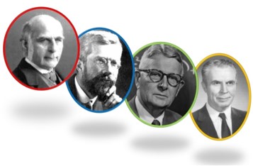
History of mixed models
Francis Galton - 1886: Regression and heritability
Ronald Fisher - 1918: Infinitesimal model (P = G + E)
Sewall Wright - 1922: Genetic relationship
Charles Henderson - 1968: BLUP using relationship
Regression and theory of heredity
Which famous scientist was Francis Galton related to?
“… the ordinary genealogical course of a race consists in a constant outgrowth from its centre, a constant dying away at its margins, and a tendency of the scanty remains of all exceptional stock to revert to that mediocrity, whence the majority of their ancestors originally sprang.” - Galton, Typical Laws of Heredity
Rediscovery of Mendelism
When did Mendel publish his laws of inheritance?
Rediscovery of Mendelism
When did Mendel publish his laws of inheritance?
1866
When was Mendelism rediscovered?
Rediscovery of Mendelism
When was Mendelism rediscovered?
1900
Which of these was not the one to rediscover Mendelism?
Hugo De Vries
William Bateson
Carl Correns
Erich von Tschermak
Rediscovery of Mendelism
Which of these was not the one to rediscover Mendelism?
Hugo De Vries
William Bateson
Carl Correns
Erich von Tschermak
Mendelians vs. Biometricians
Vigorous debates (sometimes on personal level) ensued
Biometricians
Weldon, Pearson
Mendelians
Bateson, De Vries
Mendelians vs. Biometricians
Vigorous debates (sometimes on personal level) ensued
Biometricians
Weldon, Pearson
Mendelians
Bateson, De Vries
G. Udny Yule (1902): New Phytologist 1 (9):226-27.
“Mendel’s Laws, so far from being in any way inconsistent with the Law of Ancestral Heredity, lead directly to a special case of that law.”
Further reading

Linear Regression Model
- All model terms assumed to be fixed effect
Simple linear regression
\(y = \beta_0 + \beta_1x + e\)

Multiple linear regression
\(y = \beta_0 + \beta_1x_1 + \beta_2x_2 + ... + \beta_px_p + e\)
Linear Mixed Model
Linear Mixed Model
Combination of fixed and random terms
\(y=Xb+Zu+e\)
- y = vector of observations (n)
- X = design matrix of fixed effects (n x p)
- Z = design (or incidence) matrix of random effects (n x q)
- u = vector of random effect coefficients (q)
- b = vector of fixed effect coefficients (p)
- e = vector of residuals (n)
Fixed and Random Terms
Fixed effect
- Assumed to be invariable (often you cannot recollect the data)
- Inferences are made upon the parameters
- Example: Overall mean and environmental effects
Fixed and Random Terms
Fixed effect
- Assumed to be invariable (often you cannot recollect the data)
- Inferences are made upon the parameters
- Example: Overall mean and environmental effects
Random effects
- You may not have all the levels available
- Inference are made on variance components
- Prior assumption: coefficients are normally distributed
- Example: Genetic effects
Model Notation
\(y=Xb+Zu+e\)
Assuming: \(u \sim N(0,K\sigma^{2}_{u})\) and \(e \sim N(0,I\sigma^{2}_{e})\)
- K = random effect correlation matrix (q x q)
- \(\sigma^{2}_{u}\) = random effect variance (1)
- \(\sigma^{2}_{e}\) = residual variance (1)
Model Notation
\(y=Xb+Zu+e\)
Assuming: \(u \sim N(0,K\sigma^{2}_{u})\) and \(e \sim N(0,I\sigma^{2}_{e})\)
- K = random effect correlation matrix (q x q)
- \(\sigma^{2}_{u}\) = random effect variance (1)
- \(\sigma^{2}_{e}\) = residual variance (1)
Summary:
- We know (data): \(x=\{y,X,Z,K\}\)
- We want (parameters): \(\theta=\{b,u,\sigma^{2}_{u},\sigma^{2}_{e}\}\)
- Estimation based on Gaussian likelihood: \(L(x|\theta)\)
Model Notation
Henderson’s equation
\[ \left[\begin{array}{rr} X'X & Z'X \\ X'Z & Z'Z+\lambda K^{-1} \end{array}\right] \left[\begin{array}{r} b \\ u \end{array}\right] =\left[\begin{array}{r} X'y \\ Z'y \end{array}\right] \] \(\lambda=\sigma^{2}_{e}/\sigma^{2}_{u}\) (Regularization parameters) (1)
Model notation
The mixed model can also be notated as follows
\[y=Wg+e\]
Solved as
\[[W'W+\Sigma] g = [W'y]\]
Where
\(W=[X,Z]\)
\(g=[b,u]\)
\(\Sigma = \left[\begin{array}{rr} 0 & 0 \\ 0 & \lambda K^{-1} \end{array}\right]\)
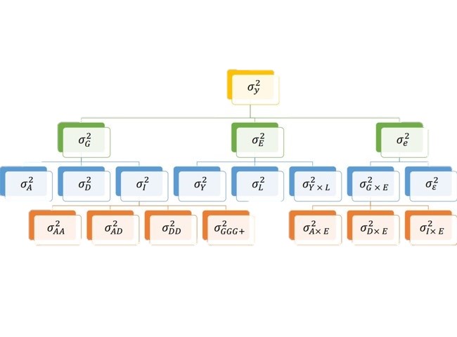
Variance decomposition
Part 2 - Applications
Selection
1 Genetic values
- BLUPs or BLUEs from replicated trials
- Captures additive and non-additive genetics together
Selection
1 Genetic values
- BLUPs or BLUEs from replicated trials
- Captures additive and non-additive genetics together
2 Breeding values
- Use pedigree information to create \(K\)
- Captures additive genetics (heritable)
- Trials not necessarily replicated
Selection
1 Genetic values
- BLUPs or BLUEs from replicated trials
- Captures additive and non-additive genetics together
2 Breeding values
- Use pedigree information to create \(K\)
- Captures additive genetics (heritable)
- Trials not necessarily replicated
3 Genomic Breeding values
- Genotypic information replaces pedigree
- Any signal: additivity, dominance and epistasis
Examples
- Example 1: Balanced data, no kinship
- Example 2: Balanced data, with kinship
Example 1
Data:
##    Env Gen Phe
## 1   E1  G1  47
## 2   E1  G2  51
## 3   E1  G3  46
## 4   E1  G4  58
## 5   E2  G1  52
## 6   E2  G2  46
## 7   E2  G3  52
## 8   E2  G4  54
## 9   E3  G1  53
## 10  E3  G2  48
## 11  E3  G3  58
## 12  E3  G4  52
Model: \(Phenotype = Environment_{(F)} + Genotype_{(R)}\)
Example 1
\[y=Wg+e\] Design matrix \(W=[X,Z]\):
##    EnvE1 EnvE2 EnvE3 GenG1 GenG2 GenG3 GenG4
## 1      1     0     0     1     0     0     0
## 2      1     0     0     0     1     0     0
## 3      1     0     0     0     0     1     0
## 4      1     0     0     0     0     0     1
## 5      0     1     0     1     0     0     0
## 6      0     1     0     0     1     0     0
## 7      0     1     0     0     0     1     0
## 8      0     1     0     0     0     0     1
## 9      0     0     1     1     0     0     0
## 10     0     0     1     0     1     0     0
## 11     0     0     1     0     0     1     0
## 12     0     0     1     0     0     0     1
Example 1
Mixed-model: \[[W'W+\Sigma] g = [W'y]\] \(W'W\):
WW = crossprod(W)
print(WW)
##       EnvE1 EnvE2 EnvE3 GenG1 GenG2 GenG3 GenG4
## EnvE1     4     0     0     1     1     1     1
## EnvE2     0     4     0     1     1     1     1
## EnvE3     0     0     4     1     1     1     1
## GenG1     1     1     1     3     0     0     0
## GenG2     1     1     1     0     3     0     0
## GenG3     1     1     1     0     0     3     0
## GenG4     1     1     1     0     0     0     3
Example 1
Mixed-model: \[[W'W+\Sigma] g = [W'y]\]
Left-hand side (\(W'W+\Sigma\)):
##       EnvE1 EnvE2 EnvE3 GenG1 GenG2 GenG3 GenG4
## EnvE1     4     0     0  1.00  1.00  1.00  1.00
## EnvE2     0     4     0  1.00  1.00  1.00  1.00
## EnvE3     0     0     4  1.00  1.00  1.00  1.00
## GenG1     1     1     1  3.17  0.00  0.00  0.00
## GenG2     1     1     1  0.00  3.17  0.00  0.00
## GenG3     1     1     1  0.00  0.00  3.17  0.00
## GenG4     1     1     1  0.00  0.00  0.00  3.17
Assuming independent individuals: \(K=I\)
Regularization: \(\lambda=\sigma^{2}_{e}/\sigma^{2}_{u}=1.64/9.56=0.17\)
Example 1
Mixed-model: \[[W'W+\Sigma] g = [W'y]\]
Right-hand side (\(W'y\)):
##       [,1]
## EnvE1  202
## EnvE2  204
## EnvE3  211
## GenG1  152
## GenG2  145
## GenG3  156
## GenG4  164
Example 1
Mixed-model: \[[W'W+\Sigma] g = [W'y]\]
We can find coefficients through least-square solution
\(g=(LHS)^{-1}(RHS)=(W'W+\Sigma)^{-1}W'y\)
##        [,1]
## EnvE1 50.50
## EnvE2 51.00
## EnvE3 52.75
## GenG1 -0.71
## GenG2 -2.92
## GenG3  0.55
## GenG4  3.08
Shrinkage
\(BLUE=\frac{w'y}{w'w}=\frac{sum}{n}\) = simple average
\(BLUP=\frac{w'y}{w'w+\lambda}=\frac{sum}{n+\lambda}\) = biased average = \(BLUE\times h^2\)
Note:
- More observations = less shrinkage
- Higher heritability = less shrinkage: \(\lambda = \frac{1- h^{2}}{h^2}\)
Example 2
If we know the relationship among individuals:
##       GenG1 GenG2 GenG3 GenG4
## GenG1  1.00  0.64  0.23  0.48
## GenG2  0.64  1.00  0.33  0.67
## GenG3  0.23  0.33  1.00  0.31
## GenG4  0.48  0.67  0.31  1.00
Example 2
Then we estimate \(\lambda K^{-1}\)
##       GenG1 GenG2 GenG3 GenG4
## GenG1  0.15 -0.09  0.00 -0.01
## GenG2 -0.09  0.22 -0.02 -0.10
## GenG3  0.00 -0.02  0.10 -0.02
## GenG4 -0.01 -0.10 -0.02  0.17
Regularization: \(\lambda=\sigma^{2}_{e}/\sigma^{2}_{u}=1.64/17.70=0.09\)
Example 2
And the left-hand side becomes
##       EnvE1 EnvE2 EnvE3 GenG1 GenG2 GenG3 GenG4
## EnvE1     4     0     0  1.00  1.00  1.00  1.00
## EnvE2     0     4     0  1.00  1.00  1.00  1.00
## EnvE3     0     0     4  1.00  1.00  1.00  1.00
## GenG1     1     1     1  3.15 -0.09  0.00 -0.01
## GenG2     1     1     1 -0.09  3.22 -0.02 -0.10
## GenG3     1     1     1  0.00 -0.02  3.10 -0.02
## GenG4     1     1     1 -0.01 -0.10 -0.02  3.17
Example 2
We can find coefficients through least-square solution
\(g=(LHS)^{-1}(RHS)=(W'W+\Sigma)^{-1}W'y\)
##        [,1]
## EnvE1 51.05
## EnvE2 51.55
## EnvE3 53.30
## GenG1 -1.32
## GenG2 -3.34
## GenG3  0.03
## GenG4  2.45
Genetic coefficients shrink more: Var(A) < Var(G)
Variance components
Expectation-Maximization REML (1977)
\(\sigma^{2}_{u} = \frac{u'K^{-1}u}{q-\lambda tr(K^{-1}C^{22})}\) and \(\sigma^{2}_{e} = \frac{e'y}{n-p}\)
Bayesian Gibbs Sampling (1993)
\(\sigma^{2}_{u} = \frac{u'K^{-1}u+S_u\nu_u}{\chi^2(q+\nu_u)}\) and \(\sigma^{2}_{e} = \frac{e'e+S_e\nu_e}{\chi^2(n+\nu_e)}\)
Ridges and Kernels
Kernel methods:
- Genetic signal is captured by the relationship matrix \(K\)
- Random effect coefficients are the breeding values (BV)
- Efficient to compute BV when \(markers \gg individuals\)
- Easy use and combine pedigree, markers and interactions
Ridge methods:
- Genetic signal is captured by the design matrix \(M\)
- Random effect coefficients are the marker effects
- Easy way to make predictions of unobserved individuals
- Enables to visualize where the QTLs are in the genome
Ridges and Kernels
Kernel
\(y=Xb+Zu+e\), \(u\sim N(0,K\sigma^2_u)\)
Ridge
\(y=Xb+Ma+e\), \(a\sim N(0,I\sigma^2_a)\)
Where
- \(M\) is the genotypic matrix, \(m_{ij}=\{0,1,2\}\)
- \(K=\alpha MM'\)
- \(u=Ma\)
- \(\sigma^2_a=\alpha\sigma^2_u\)
Ridges and Kernels
Kernel model
\[ \left[\begin{array}{rr} X'X & Z'X \\ X'Z & Z'Z+K^{-1}(\sigma^2_e/\sigma^2_u) \end{array}\right] \left[\begin{array}{r} b \\ u \end{array}\right] =\left[\begin{array}{r} X'y \\ Z'y \end{array}\right] \]
Ridge model
\[ \left[\begin{array}{rr} X'X & M'X \\ X'M & M'M+I^{-1}(\sigma^2_e/\sigma^2_a) \end{array}\right] \left[\begin{array}{r} b \\ a \end{array}\right] =\left[\begin{array}{r} X'y \\ M'y \end{array}\right] \]
Both models capture same genetic signal (de los Campos 2015)
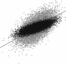
Ridges and Kernels
K = tcrossprod(M)/ncol(M)
GBLUP = reml(y=y,K=K); Kernel_GEBV = GBLUP$EBV
RRBLUP = reml(y=y,Z=M); Ridge_GEBV = M%*%RRBLUP$EBV
plot(Kernel_GEBV,Ridge_GEBV, main='Comparing results')

Mixed models in plant breeding
- Variance components and heritability (Johnson and Thompson 1994)
- Trait associations (Gianola and Sorensen 2014)
- Estimation of genetic and breeding values (Piepho et al 2008)
- Prediction of unphenotyped lines (de los Campos et al 2013)
- Selection index (Wientjes et al. 2016)
- Genome-wide association analysis (Yang et al 2014)
- All sorts of inference (Robinson 1991)
- One hundred years of statistical developments (Gianola and Rosa 2014)