Multiple linear regression

library(car)
library(MASS)
library(psych)

Loading and describing data

data(Boston)
data_ori <- Boston
describe(data_ori)

##         vars   n   mean     sd median trimmed    mad    min    max  range  skew
## crim       1 506   3.61   8.60   0.26    1.68   0.33   0.01  88.98  88.97  5.19
## zn         2 506  11.36  23.32   0.00    5.08   0.00   0.00 100.00 100.00  2.21
## indus      3 506  11.14   6.86   9.69   10.93   9.37   0.46  27.74  27.28  0.29
## chas       4 506   0.07   0.25   0.00    0.00   0.00   0.00   1.00   1.00  3.39
## nox        5 506   0.55   0.12   0.54    0.55   0.13   0.38   0.87   0.49  0.72
## rm         6 506   6.28   0.70   6.21    6.25   0.51   3.56   8.78   5.22  0.40
## age        7 506  68.57  28.15  77.50   71.20  28.98   2.90 100.00  97.10 -0.60
## dis        8 506   3.80   2.11   3.21    3.54   1.91   1.13  12.13  11.00  1.01
## rad        9 506   9.55   8.71   5.00    8.73   2.97   1.00  24.00  23.00  1.00
## tax       10 506 408.24 168.54 330.00  400.04 108.23 187.00 711.00 524.00  0.67
## ptratio   11 506  18.46   2.16  19.05   18.66   1.70  12.60  22.00   9.40 -0.80
## black     12 506 356.67  91.29 391.44  383.17   8.09   0.32 396.90 396.58 -2.87
## lstat     13 506  12.65   7.14  11.36   11.90   7.11   1.73  37.97  36.24  0.90
## medv      14 506  22.53   9.20  21.20   21.56   5.93   5.00  50.00  45.00  1.10
##         kurtosis   se
## crim       36.60 0.38
## zn          3.95 1.04
## indus      -1.24 0.30
## chas        9.48 0.01
## nox        -0.09 0.01
## rm          1.84 0.03
## age        -0.98 1.25
## dis         0.46 0.09
## rad        -0.88 0.39
## tax        -1.15 7.49
## ptratio    -0.30 0.10
## black       7.10 4.06
## lstat       0.46 0.32
## medv        1.45 0.41

summary(data_ori)

##       crim                zn             indus            chas        
##  Min.   : 0.00632   Min.   :  0.00   Min.   : 0.46   Min.   :0.00000  
##  1st Qu.: 0.08205   1st Qu.:  0.00   1st Qu.: 5.19   1st Qu.:0.00000  
##  Median : 0.25651   Median :  0.00   Median : 9.69   Median :0.00000  
##  Mean   : 3.61352   Mean   : 11.36   Mean   :11.14   Mean   :0.06917  
##  3rd Qu.: 3.67708   3rd Qu.: 12.50   3rd Qu.:18.10   3rd Qu.:0.00000  
##  Max.   :88.97620   Max.   :100.00   Max.   :27.74   Max.   :1.00000  
##       nox               rm             age              dis        
##  Min.   :0.3850   Min.   :3.561   Min.   :  2.90   Min.   : 1.130  
##  1st Qu.:0.4490   1st Qu.:5.886   1st Qu.: 45.02   1st Qu.: 2.100  
##  Median :0.5380   Median :6.208   Median : 77.50   Median : 3.207  
##  Mean   :0.5547   Mean   :6.285   Mean   : 68.57   Mean   : 3.795  
##  3rd Qu.:0.6240   3rd Qu.:6.623   3rd Qu.: 94.08   3rd Qu.: 5.188  
##  Max.   :0.8710   Max.   :8.780   Max.   :100.00   Max.   :12.127  
##       rad              tax           ptratio          black       
##  Min.   : 1.000   Min.   :187.0   Min.   :12.60   Min.   :  0.32  
##  1st Qu.: 4.000   1st Qu.:279.0   1st Qu.:17.40   1st Qu.:375.38  
##  Median : 5.000   Median :330.0   Median :19.05   Median :391.44  
##  Mean   : 9.549   Mean   :408.2   Mean   :18.46   Mean   :356.67  
##  3rd Qu.:24.000   3rd Qu.:666.0   3rd Qu.:20.20   3rd Qu.:396.23  
##  Max.   :24.000   Max.   :711.0   Max.   :22.00   Max.   :396.90  
##      lstat            medv      
##  Min.   : 1.73   Min.   : 5.00  
##  1st Qu.: 6.95   1st Qu.:17.02  
##  Median :11.36   Median :21.20  
##  Mean   :12.65   Mean   :22.53  
##  3rd Qu.:16.95   3rd Qu.:25.00  
##  Max.   :37.97   Max.   :50.00

Create table 1

library(boot) 
library(table1)
table1(~ . , data=data_ori)

	Overall (N=506)
crim
Mean (SD)	3.61 (8.60)
Median [Min, Max]	0.257 [0.00632, 89.0]
zn
Mean (SD)	11.4 (23.3)
Median [Min, Max]	0 [0, 100]
indus
Mean (SD)	11.1 (6.86)
Median [Min, Max]	9.69 [0.460, 27.7]
chas
Mean (SD)	0.0692 (0.254)
Median [Min, Max]	0 [0, 1.00]
nox
Mean (SD)	0.555 (0.116)
Median [Min, Max]	0.538 [0.385, 0.871]
rm
Mean (SD)	6.28 (0.703)
Median [Min, Max]	6.21 [3.56, 8.78]
age
Mean (SD)	68.6 (28.1)
Median [Min, Max]	77.5 [2.90, 100]
dis
Mean (SD)	3.80 (2.11)
Median [Min, Max]	3.21 [1.13, 12.1]
rad
Mean (SD)	9.55 (8.71)
Median [Min, Max]	5.00 [1.00, 24.0]
tax
Mean (SD)	408 (169)
Median [Min, Max]	330 [187, 711]
ptratio
Mean (SD)	18.5 (2.16)
Median [Min, Max]	19.1 [12.6, 22.0]
black
Mean (SD)	357 (91.3)
Median [Min, Max]	391 [0.320, 397]
lstat
Mean (SD)	12.7 (7.14)
Median [Min, Max]	11.4 [1.73, 38.0]
medv
Mean (SD)	22.5 (9.20)
Median [Min, Max]	21.2 [5.00, 50.0]

Missingness checking

library(mice)
md.pattern(data_ori)

##  /\     /\
## {  `---'  }
## {  O   O  }
## ==>  V <==  No need for mice. This data set is completely observed.
##  \  \|/  /
##   `-----'

##     crim zn indus chas nox rm age dis rad tax ptratio black lstat medv  
## 506    1  1     1    1   1  1   1   1   1   1       1     1     1    1 0
##        0  0     0    0   0  0   0   0   0   0       0     0     0    0 0

Exploratory data analysis

-correlation matrix

library(psych)
pairs.panels(data_ori)

histogram

library(DataExplorer)
plot_histogram(data_ori)

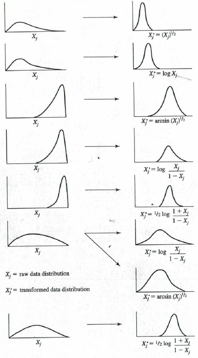
Transformations

transformation (based on the following rule) then histogram

library(tidyverse)
data_trans = data_ori %>%  mutate(age= sqrt(max(age)+1-age),
                         black= log10(max(black)+1-black),
                         crim= log10(crim),
                         dis= sqrt(dis)   )
plot_histogram(data_trans)

# pairs.panels(data2)

! How to transform data for normality.

check linearity between y and x

attach(data_trans)
plot(medv, rm)

plot(medv,lstat)

plot(medv,age)

plot(medv, black)

plot(medv,crim)

Data imputation and normalization

For original”data”

compiling knnimpute model (see machine learning section)

library(caret)
# Create the knn imputation model on the training data
y=data_ori$medv
preProcess_missingdata_model <- preProcess(data_ori , method='knnImpute')
preProcess_missingdata_model

## Created from 506 samples and 14 variables
## 
## Pre-processing:
##   - centered (14)
##   - ignored (0)
##   - 5 nearest neighbor imputation (14)
##   - scaled (14)

check missingness

# Use the imputation model to predict the values of missing data points
library(RANN)  # required for knnInpute
data_ori  <- predict(preProcess_missingdata_model, newdata = data_ori )
anyNA(data_ori )

## [1] FALSE

data_ori$medv <- y

For transformed “data2”

compiling knnimpute model (see machine learning section)

library(caret)
y2=data_trans$medv
# Create the knn imputation model on the training data
preProcess_missingdata_model2 <- preProcess(data_trans , method='knnImpute')
preProcess_missingdata_model2

## Created from 506 samples and 14 variables
## 
## Pre-processing:
##   - centered (14)
##   - ignored (0)
##   - 5 nearest neighbor imputation (14)
##   - scaled (14)

check missingness

# Use the imputation model to predict the values of missing data points
library(RANN)  # required for knnInpute
data_trans  <- predict(preProcess_missingdata_model2, newdata = data_trans )
anyNA(data_trans )

## [1] FALSE

data_trans$medv <- y2

Generate dummy variables

also can do using as.factor function for predictors x

Spliting data into trainning data and test data

by using caret package (test data for external validation)

# Create the training and test datasets
set.seed(123)
# for original data 
# Step 1: Get row numbers for the training data
trainRowNumbers <- createDataPartition(data_ori$medv, p=0.8, list=FALSE)

# Step 2: Create the training  dataset
data  <- data_ori[trainRowNumbers,]

# Step 3: Create the test dataset
testdata  <- data_ori[-trainRowNumbers,]

# for transformed data
# Step 1: Get row numbers for the training data
trainRowNumbers2 <- createDataPartition(data_trans$medv, p=0.8, list=FALSE)

# Step 2: Create the training  dataset
data2 <- data_trans[trainRowNumbers2,]

# Step 3: Create the test dataset
testdata2 <- data_trans[-trainRowNumbers2,]

Step regression

model_o = lm(  medv ~.  , data=data2)
step(model_o,direction = "both")

## Start:  AIC=1281.15
## medv ~ crim + zn + indus + chas + nox + rm + age + dis + rad + 
##     tax + ptratio + black + lstat
## 
##           Df Sum of Sq     RSS    AIC
## - black    1      0.17  8847.0 1279.2
## - age      1      7.07  8853.9 1279.5
## - crim     1     14.36  8861.2 1279.8
## - indus    1     24.08  8870.9 1280.3
## <none>                  8846.8 1281.2
## - rad      1    103.22  8950.0 1283.9
## - tax      1    156.33  9003.1 1286.3
## - zn       1    198.34  9045.2 1288.2
## - chas     1    251.31  9098.1 1290.5
## - nox      1    692.00  9538.8 1309.8
## - ptratio  1    840.04  9686.9 1316.1
## - rm       1    965.90  9812.7 1321.3
## - dis      1   1349.41 10196.2 1336.9
## - lstat    1   2766.14 11613.0 1389.9
## 
## Step:  AIC=1279.16
## medv ~ crim + zn + indus + chas + nox + rm + age + dis + rad + 
##     tax + ptratio + lstat
## 
##           Df Sum of Sq     RSS    AIC
## - age      1      7.15  8854.1 1277.5
## - crim     1     14.32  8861.3 1277.8
## - indus    1     24.52  8871.5 1278.3
## <none>                  8847.0 1279.2
## + black    1      0.17  8846.8 1281.2
## - rad      1    103.72  8950.7 1281.9
## - tax      1    157.40  9004.4 1284.3
## - zn       1    198.20  9045.2 1286.2
## - chas     1    251.25  9098.2 1288.6
## - nox      1    695.37  9542.4 1308.0
## - ptratio  1    850.76  9697.7 1314.5
## - rm       1    966.99  9814.0 1319.4
## - dis      1   1375.04 10222.0 1336.0
## - lstat    1   2770.28 11617.3 1388.0
## 
## Step:  AIC=1277.49
## medv ~ crim + zn + indus + chas + nox + rm + dis + rad + tax + 
##     ptratio + lstat
## 
##           Df Sum of Sq     RSS    AIC
## - crim     1     18.36  8872.5 1276.3
## - indus    1     25.56  8879.7 1276.7
## <none>                  8854.1 1277.5
## + age      1      7.15  8847.0 1279.2
## + black    1      0.26  8853.9 1279.5
## - rad      1     97.20  8951.3 1279.9
## - tax      1    152.93  9007.1 1282.5
## - zn       1    196.76  9050.9 1284.4
## - chas     1    255.17  9109.3 1287.0
## - nox      1    694.68  9548.8 1306.2
## - ptratio  1    843.66  9697.8 1312.5
## - rm       1   1023.40  9877.5 1320.0
## - dis      1   1633.60 10487.7 1344.4
## - lstat    1   2978.57 11832.7 1393.5
## 
## Step:  AIC=1276.33
## medv ~ zn + indus + chas + nox + rm + dis + rad + tax + ptratio + 
##     lstat
## 
##           Df Sum of Sq     RSS    AIC
## - indus    1     21.92  8894.4 1275.3
## <none>                  8872.5 1276.3
## + crim     1     18.36  8854.1 1277.5
## + age      1     11.19  8861.3 1277.8
## + black    1      0.13  8872.4 1278.3
## - tax      1    158.39  9030.9 1281.5
## - zn       1    180.19  9052.7 1282.5
## - rad      1    212.19  9084.7 1284.0
## - chas     1    249.50  9122.0 1285.6
## - nox      1    689.33  9561.8 1304.8
## - ptratio  1    873.78  9746.3 1312.6
## - rm       1   1025.43  9897.9 1318.8
## - dis      1   1701.37 10573.9 1345.7
## - lstat    1   2996.77 11869.3 1392.8
## 
## Step:  AIC=1275.34
## medv ~ zn + chas + nox + rm + dis + rad + tax + ptratio + lstat
## 
##           Df Sum of Sq     RSS    AIC
## <none>                  8894.4 1275.3
## + indus    1     21.92  8872.5 1276.3
## + crim     1     14.72  8879.7 1276.7
## + age      1     11.89  8882.5 1276.8
## + black    1      0.00  8894.4 1277.3
## - zn       1    206.52  9100.9 1282.7
## - chas     1    237.50  9131.9 1284.1
## - tax      1    281.42  9175.8 1286.0
## - rad      1    293.27  9187.7 1286.5
## - nox      1    800.54  9695.0 1308.4
## - ptratio  1    929.05  9823.5 1313.8
## - rm       1   1083.34  9977.8 1320.1
## - dis      1   1706.94 10601.4 1344.8
## - lstat    1   3024.07 11918.5 1392.5

## 
## Call:
## lm(formula = medv ~ zn + chas + nox + rm + dis + rad + tax + 
##     ptratio + lstat, data = data2)
## 
## Coefficients:
## (Intercept)           zn         chas          nox           rm          dis  
##      22.509        1.016        0.759       -2.764        2.176       -3.970  
##         rad          tax      ptratio        lstat  
##       2.119       -2.317       -1.991       -4.224

# summary(step(model_o,direction = "both"))

Create a model after selecting variables

model_trasf <- lm(formula = medv ~ zn + chas + nox + rm + dis + rad + tax + 
    ptratio + lstat, data = data2)
summary(model_trasf)

## 
## Call:
## lm(formula = medv ~ zn + chas + nox + rm + dis + rad + tax + 
##     ptratio + lstat, data = data2)
## 
## Residuals:
##      Min       1Q   Median       3Q      Max 
## -13.2923  -2.4690  -0.5086   1.6269  24.5813 
## 
## Coefficients:
##             Estimate Std. Error t value Pr(>|t|)    
## (Intercept)  22.5090     0.2352  95.718  < 2e-16 ***
## zn            1.0161     0.3347   3.036 0.002554 ** 
## chas          0.7590     0.2331   3.256 0.001227 ** 
## nox          -2.7640     0.4624  -5.978 5.05e-09 ***
## rm            2.1760     0.3129   6.954 1.47e-11 ***
## dis          -3.9697     0.4548  -8.729  < 2e-16 ***
## rad           2.1194     0.5858   3.618 0.000335 ***
## tax          -2.3171     0.6538  -3.544 0.000441 ***
## ptratio      -1.9909     0.3092  -6.440 3.47e-10 ***
## lstat        -4.2244     0.3636 -11.618  < 2e-16 ***
## ---
## Signif. codes:  0 '***' 0.001 '**' 0.01 '*' 0.05 '.' 0.1 ' ' 1
## 
## Residual standard error: 4.733 on 397 degrees of freedom
## Multiple R-squared:  0.7187, Adjusted R-squared:  0.7123 
## F-statistic: 112.7 on 9 and 397 DF,  p-value: < 2.2e-16

Multicollinearity checking

vif(model_trasf)

##       zn     chas      nox       rm      dis      rad      tax  ptratio 
## 2.024269 1.044796 4.074241 1.721080 3.759267 6.008751 7.469414 1.743359 
##    lstat 
## 2.372125

Plot model to check assumptions

plot(model_trasf)

histogram of residuals

resid<- model_trasf$residuals
hist(resid)

F test of model

anova(model_trasf)

## Analysis of Variance Table
## 
## Response: medv
##            Df Sum Sq Mean Sq F value    Pr(>F)    
## zn          1 4019.0  4019.0 179.388 < 2.2e-16 ***
## chas        1 1011.6  1011.6  45.151 6.349e-11 ***
## nox         1 2785.8  2785.8 124.344 < 2.2e-16 ***
## rm          1 8487.1  8487.1 378.818 < 2.2e-16 ***
## dis         1  951.8   951.8  42.482 2.168e-10 ***
## rad         1  558.9   558.9  24.944 8.857e-07 ***
## tax         1  767.9   767.9  34.274 1.004e-08 ***
## ptratio     1 1119.4  1119.4  49.964 7.090e-12 ***
## lstat       1 3024.1  3024.1 134.978 < 2.2e-16 ***
## Residuals 397 8894.4    22.4                      
## ---
## Signif. codes:  0 '***' 0.001 '**' 0.01 '*' 0.05 '.' 0.1 ' ' 1

coefficients

coef(summary(model_trasf))

##               Estimate Std. Error    t value      Pr(>|t|)
## (Intercept) 22.5089571  0.2351584  95.718273 2.288696e-276
## zn           1.0160975  0.3346703   3.036115  2.554477e-03
## chas         0.7589909  0.2331142   3.255876  1.227473e-03
## nox         -2.7639762  0.4623875  -5.977619  5.046096e-09
## rm           2.1760130  0.3129267   6.953747  1.471198e-11
## dis         -3.9697228  0.4547944  -8.728609  7.226931e-17
## rad          2.1193795  0.5857829   3.618029  3.351805e-04
## tax         -2.3171470  0.6537962  -3.544143  4.407963e-04
## ptratio     -1.9908948  0.3091666  -6.439552  3.465747e-10
## lstat       -4.2244121  0.3636086 -11.618019  4.644137e-27

confidence interval

confint(model_trasf)

##                  2.5 %    97.5 %
## (Intercept) 22.0466457 22.971269
## zn           0.3581500  1.674045
## chas         0.3006983  1.217284
## nox         -3.6730103 -1.854942
## rm           1.5608125  2.791213
## dis         -4.8638292 -3.075616
## rad          0.9677553  3.271004
## tax         -3.6024824 -1.031811
## ptratio     -2.5987032 -1.383086
## lstat       -4.9392512 -3.509573

Add polynomial of quadratic term

rm and lstat

model_trasf_poly <- lm(formula = medv ~ zn + chas + nox +  I(rm^2) + dis + rad + tax + 
    ptratio +   I(lstat^2), data = data2)
summary(model_trasf_poly)

## 
## Call:
## lm(formula = medv ~ zn + chas + nox + I(rm^2) + dis + rad + tax + 
##     ptratio + I(lstat^2), data = data2)
## 
## Residuals:
##      Min       1Q   Median       3Q      Max 
## -19.0736  -3.4029  -0.6212   2.8340  29.4942 
## 
## Coefficients:
##             Estimate Std. Error t value Pr(>|t|)    
## (Intercept)  22.2859     0.3526  63.212  < 2e-16 ***
## zn            1.5524     0.4096   3.790 0.000174 ***
## chas          0.9570     0.2834   3.377 0.000805 ***
## nox          -4.4962     0.5455  -8.242 2.50e-15 ***
## I(rm^2)       1.5313     0.1589   9.637  < 2e-16 ***
## dis          -3.3186     0.5644  -5.880 8.69e-09 ***
## rad           3.0529     0.7024   4.346 1.76e-05 ***
## tax          -3.6647     0.7861  -4.662 4.28e-06 ***
## ptratio      -2.6800     0.3706  -7.232 2.47e-12 ***
## I(lstat^2)   -1.3170     0.1918  -6.865 2.56e-11 ***
## ---
## Signif. codes:  0 '***' 0.001 '**' 0.01 '*' 0.05 '.' 0.1 ' ' 1
## 
## Residual standard error: 5.763 on 397 degrees of freedom
## Multiple R-squared:  0.583,  Adjusted R-squared:  0.5735 
## F-statistic: 61.67 on 9 and 397 DF,  p-value: < 2.2e-16

Add interaction terms

rm and lstat
R2 >0.7 indicates a good fit of the model

model_trasf_term <- lm(formula = medv ~ zn + chas + nox +  (rm*  lstat) + dis + rad + tax + 
    ptratio  , data = data2)
summary(model_trasf_term)

## 
## Call:
## lm(formula = medv ~ zn + chas + nox + (rm * lstat) + dis + rad + 
##     tax + ptratio, data = data2)
## 
## Residuals:
##      Min       1Q   Median       3Q      Max 
## -19.4595  -2.3458  -0.2389   1.7950  26.6992 
## 
## Coefficients:
##             Estimate Std. Error t value Pr(>|t|)    
## (Intercept)  21.4297     0.2379  90.060  < 2e-16 ***
## zn            0.5221     0.3046   1.714 0.087296 .  
## chas          0.6538     0.2095   3.120 0.001941 ** 
## nox          -2.0295     0.4218  -4.812 2.13e-06 ***
## rm            1.6459     0.2860   5.754 1.75e-08 ***
## lstat        -5.8715     0.3669 -16.002  < 2e-16 ***
## dis          -3.1810     0.4161  -7.645 1.60e-13 ***
## rad           1.9251     0.5262   3.658 0.000288 ***
## tax          -1.9187     0.5883  -3.261 0.001205 ** 
## ptratio      -1.5554     0.2811  -5.534 5.70e-08 ***
## rm:lstat     -1.8202     0.1852  -9.830  < 2e-16 ***
## ---
## Signif. codes:  0 '***' 0.001 '**' 0.01 '*' 0.05 '.' 0.1 ' ' 1
## 
## Residual standard error: 4.249 on 396 degrees of freedom
## Multiple R-squared:  0.7739, Adjusted R-squared:  0.7682 
## F-statistic: 135.5 on 10 and 396 DF,  p-value: < 2.2e-16

plot(model_trasf_term)

Robust regression

robust_model_term <- rlm(medv ~ zn + chas + nox +  (rm*  lstat) + dis + rad + tax + 
    ptratio  , data = data2)
summary(robust_model_term)

## 
## Call: rlm(formula = medv ~ zn + chas + nox + (rm * lstat) + dis + rad + 
##     tax + ptratio, data = data2)
## Residuals:
##       Min        1Q    Median        3Q       Max 
## -20.90999  -1.74873  -0.09845   1.92931  33.87244 
## 
## Coefficients:
##             Value    Std. Error t value 
## (Intercept)  20.9624   0.1656   126.5763
## zn            0.1998   0.2120     0.9424
## chas          0.5198   0.1458     3.5643
## nox          -1.3458   0.2935    -4.5846
## rm            2.8773   0.1991    14.4524
## lstat        -4.5706   0.2554   -17.8979
## dis          -1.9208   0.2896    -6.6326
## rad           0.9005   0.3663     2.4586
## tax          -1.7199   0.4095    -4.2004
## ptratio      -1.2451   0.1956    -6.3652
## rm:lstat     -1.9899   0.1289   -15.4398
## 
## Residual standard error: 2.698 on 396 degrees of freedom

Create a model before transforming data

model_trasf_orig <- lm(formula = medv ~ zn + chas + nox + rm + dis + rad + tax + 
    ptratio + lstat, data = data)
summary(model_trasf_orig)

## 
## Call:
## lm(formula = medv ~ zn + chas + nox + rm + dis + rad + tax + 
##     ptratio + lstat, data = data)
## 
## Residuals:
##     Min      1Q  Median      3Q     Max 
## -14.219  -2.729  -0.463   1.920  25.992 
## 
## Coefficients:
##             Estimate Std. Error t value Pr(>|t|)    
## (Intercept)  22.5094     0.2430  92.619  < 2e-16 ***
## zn            0.8232     0.3754   2.193 0.028904 *  
## chas          0.6582     0.2412   2.728 0.006652 ** 
## nox          -1.9351     0.4727  -4.093 5.15e-05 ***
## rm            2.3985     0.3128   7.668 1.36e-13 ***
## dis          -2.9289     0.4565  -6.416 3.99e-10 ***
## rad           2.2109     0.6348   3.483 0.000551 ***
## tax          -2.1880     0.6896  -3.173 0.001627 ** 
## ptratio      -2.0274     0.3254  -6.230 1.19e-09 ***
## lstat        -4.3534     0.3844 -11.325  < 2e-16 ***
## ---
## Signif. codes:  0 '***' 0.001 '**' 0.01 '*' 0.05 '.' 0.1 ' ' 1
## 
## Residual standard error: 4.895 on 397 degrees of freedom
## Multiple R-squared:  0.7212, Adjusted R-squared:  0.7149 
## F-statistic: 114.1 on 9 and 397 DF,  p-value: < 2.2e-16

non nest models comparisons

AIC(model_trasf,model_trasf_orig)

##                  df      AIC
## model_trasf      11 2432.353
## model_trasf_orig 11 2459.780

K-fold cross validation

to make sure which model is better

# install.packages("DAAG")
library(DAAG)
 
set.seed(123)
model_trasf_term_cv <- glm( medv ~ zn + chas + nox +  (rm*  lstat) + dis + rad + tax + 
    ptratio  , data = data2)
cv.err  <- cv.glm(data2, model_trasf_term_cv, K = 10)$delta
cv.err

## [1] 19.24588 19.15400

Nonnest models comparisons

AIC(model_trasf_term,model_trasf,model_trasf_orig,model_trasf_poly)

##                  df      AIC
## model_trasf_term 12 2345.492
## model_trasf      11 2432.353
## model_trasf_orig 11 2459.780
## model_trasf_poly 11 2592.584

# interaction, transformation, original, polynomial by order (`data` has been normalized but not `data2`)

plot the final model and check the model assumption

posterior predictive check, linearity, homogeneity of variance, influential points, colinearity, and normality of residuals

# install.packages("performance")
library(performance)
check_model(model_trasf_term)

Create forest plot for coefficients

library(sjPlot)

## Registered S3 methods overwritten by 'effectsize':
##   method              from      
##   standardize.Surv    datawizard
##   standardize.bcplm   datawizard
##   standardize.clm2    datawizard
##   standardize.default datawizard
##   standardize.mediate datawizard
##   standardize.wbgee   datawizard
##   standardize.wbm     datawizard

## #refugeeswelcome

plot_model(model_trasf_term, show.values = TRUE, value.offset = 0.4)

Relative Importance

provides measures of relative importance

library(relaimpo)
# calc.relimp(fit,type=c("lmg","last","first","pratt"),
#    rela=TRUE)
# Bootstrap Measures of Relative Importance (1000 samples)
boot <- boot.relimp(model_trasf_term, b = 10, type =c("lmg" ), rank = TRUE,
                    # type =c("lmg","last","first","pratt")
  diff = TRUE, rela = TRUE)
booteval.relimp(boot) # print result

## Warning in norm.inter(t, alpha): extreme order statistics used as endpoints

## Warning in norm.inter(t, alpha): extreme order statistics used as endpoints

## Warning in norm.inter(t, alpha): extreme order statistics used as endpoints

## Warning in norm.inter(t, alpha): extreme order statistics used as endpoints

## Warning in norm.inter(t, alpha): extreme order statistics used as endpoints

## Warning in norm.inter(t, alpha): extreme order statistics used as endpoints

## Warning in norm.inter(t, alpha): extreme order statistics used as endpoints

## Warning in norm.inter(t, alpha): extreme order statistics used as endpoints

## Warning in norm.inter(t, alpha): extreme order statistics used as endpoints

## Warning in norm.inter(t, alpha): extreme order statistics used as endpoints

## Warning in norm.inter(t, alpha): extreme order statistics used as endpoints

## Warning in norm.inter(t, alpha): extreme order statistics used as endpoints

## Warning in norm.inter(t, alpha): extreme order statistics used as endpoints

## Warning in norm.inter(t, alpha): extreme order statistics used as endpoints

## Warning in norm.inter(t, alpha): extreme order statistics used as endpoints

## Warning in norm.inter(t, alpha): extreme order statistics used as endpoints

## Warning in norm.inter(t, alpha): extreme order statistics used as endpoints

## Warning in norm.inter(t, alpha): extreme order statistics used as endpoints

## Warning in norm.inter(t, alpha): extreme order statistics used as endpoints

## Warning in norm.inter(t, alpha): extreme order statistics used as endpoints

## Warning in norm.inter(t, alpha): extreme order statistics used as endpoints

## Warning in norm.inter(t, alpha): extreme order statistics used as endpoints

## Warning in norm.inter(t, alpha): extreme order statistics used as endpoints

## Warning in norm.inter(t, alpha): extreme order statistics used as endpoints

## Warning in norm.inter(t, alpha): extreme order statistics used as endpoints

## Warning in norm.inter(t, alpha): extreme order statistics used as endpoints

## Warning in norm.inter(t, alpha): extreme order statistics used as endpoints

## Warning in norm.inter(t, alpha): extreme order statistics used as endpoints

## Warning in norm.inter(t, alpha): extreme order statistics used as endpoints

## Warning in norm.inter(t, alpha): extreme order statistics used as endpoints

## Warning in norm.inter(t, alpha): extreme order statistics used as endpoints

## Warning in norm.inter(t, alpha): extreme order statistics used as endpoints

## Warning in norm.inter(t, alpha): extreme order statistics used as endpoints

## Warning in norm.inter(t, alpha): extreme order statistics used as endpoints

## Warning in norm.inter(t, alpha): extreme order statistics used as endpoints

## Warning in norm.inter(t, alpha): extreme order statistics used as endpoints

## Warning in norm.inter(t, alpha): extreme order statistics used as endpoints

## Warning in norm.inter(t, alpha): extreme order statistics used as endpoints

## Warning in norm.inter(t, alpha): extreme order statistics used as endpoints

## Warning in norm.inter(t, alpha): extreme order statistics used as endpoints

## Warning in norm.inter(t, alpha): extreme order statistics used as endpoints

## Warning in norm.inter(t, alpha): extreme order statistics used as endpoints

## Warning in norm.inter(t, alpha): extreme order statistics used as endpoints

## Warning in norm.inter(t, alpha): extreme order statistics used as endpoints

## Warning in norm.inter(t, alpha): extreme order statistics used as endpoints

## Warning in norm.inter(t, alpha): extreme order statistics used as endpoints

## Warning in norm.inter(t, alpha): extreme order statistics used as endpoints

## Warning in norm.inter(t, alpha): extreme order statistics used as endpoints

## Warning in norm.inter(t, alpha): extreme order statistics used as endpoints

## Warning in norm.inter(t, alpha): extreme order statistics used as endpoints

## Warning in norm.inter(t, alpha): extreme order statistics used as endpoints

## Warning in norm.inter(t, alpha): extreme order statistics used as endpoints

## Warning in norm.inter(t, alpha): extreme order statistics used as endpoints

## Warning in norm.inter(t, alpha): extreme order statistics used as endpoints

## Warning in norm.inter(t, alpha): extreme order statistics used as endpoints

## Warning in norm.inter(t, alpha): extreme order statistics used as endpoints

## Warning in norm.inter(t, alpha): extreme order statistics used as endpoints

## Warning in norm.inter(t, alpha): extreme order statistics used as endpoints

## Warning in norm.inter(t, alpha): extreme order statistics used as endpoints

## Warning in norm.inter(t, alpha): extreme order statistics used as endpoints

## Warning in norm.inter(t, alpha): extreme order statistics used as endpoints

## Warning in norm.inter(t, alpha): extreme order statistics used as endpoints

## Warning in norm.inter(t, alpha): extreme order statistics used as endpoints

## Warning in norm.inter(t, alpha): extreme order statistics used as endpoints

## Warning in norm.inter(t, alpha): extreme order statistics used as endpoints

## Response variable: medv 
## Total response variance: 77.88147 
## Analysis based on 407 observations 
## 
## 10 Regressors: 
## zn chas nox rm lstat dis rad tax ptratio rm:lstat 
## Proportion of variance explained by model: 77.39%
## Metrics are normalized to sum to 100% (rela=TRUE). 
## 
## Relative importance metrics: 
## 
##                 lmg
## zn       0.03220843
## chas     0.01925573
## nox      0.05753222
## rm       0.24841214
## lstat    0.32582422
## dis      0.04647715
## rad      0.03216196
## tax      0.05940953
## ptratio  0.09003437
## rm:lstat 0.08868423
## 
## Average coefficients for different model sizes: 
## 
##                  1X        2Xs        3Xs        4Xs        5Xs        6Xs
## zn        3.1505046  2.1309586  1.5419108  1.1885764  0.9622432  0.8066737
## chas      1.4317561  1.3828980  1.2922217  1.1827563  1.0710746  0.9666952
## nox      -3.6683140 -2.8590532 -2.3987148 -2.1635246 -2.0628637 -2.0336275
## rm        5.8715576  5.1812470  4.6686609  4.2214027  3.7902531  3.3584729
## lstat    -6.3961998 -6.2413211 -6.1543204 -6.0962610 -6.0505503 -6.0111059
## dis       2.3495853  0.6106749 -0.5986185 -1.4554886 -2.0655023 -2.4944977
## rad      -3.2090101 -1.5469225 -0.4505596  0.2850626  0.7884232  1.1408255
## tax      -4.1727995 -3.6061521 -3.1776467 -2.8413999 -2.5683300 -2.3434564
## ptratio  -4.2048171 -3.4233285 -2.9476391 -2.6199136 -2.3633992 -2.1469790
## rm:lstat -0.7386853 -1.0072327 -1.1975350 -1.3430505 -1.4610987 -1.5602846
##                 7Xs        8Xs        9Xs       10Xs
## zn        0.6942682  0.6122971  0.5558327  0.5221292
## chas      0.8734919  0.7916003  0.7191770  0.6537613
## nox      -2.0351844 -2.0434312 -2.0444974 -2.0294702
## rm        2.9235837  2.4886854  2.0599352  1.6458985
## lstat    -5.9756419 -5.9424093 -5.9088868 -5.8714971
## dis      -2.7882468 -2.9825750 -3.1064663 -3.1809633
## rad       1.3969994  1.5963587  1.7666711  1.9250667
## tax      -2.1625306 -2.0281734 -1.9455332 -1.9186629
## ptratio  -1.9610124 -1.8027959 -1.6694147 -1.5553973
## rm:lstat -1.6447082 -1.7160362 -1.7745576 -1.8202278
## 
##  
##  Confidence interval information ( 10 bootstrap replicates, bty= perc ): 
## Relative Contributions with confidence intervals: 
##  
##                                    Lower  Upper
##              percentage 0.95       0.95   0.95  
## zn.lmg       0.0322     _______HIJ 0.0202 0.0358
## chas.lmg     0.0193     _____FGHIJ 0.0016 0.0512
## nox.lmg      0.0575     ____EFG___ 0.0432 0.0707
## rm.lmg       0.2484     AB________ 0.1929 0.3313
## lstat.lmg    0.3258     AB________ 0.2627 0.3840
## dis.lmg      0.0465     _____FGHIJ 0.0288 0.0545
## rad.lmg      0.0322     ______GHIJ 0.0213 0.0457
## tax.lmg      0.0594     ___DEFG___ 0.0476 0.0784
## ptratio.lmg  0.0900     __CD______ 0.0712 0.1159
## rm:lstat.lmg 0.0887     __CDEF____ 0.0614 0.1112
## 
## Letters indicate the ranks covered by bootstrap CIs. 
## (Rank bootstrap confidence intervals always obtained by percentile method) 
## CAUTION: Bootstrap confidence intervals can be somewhat liberal. 
## 
##  
##  Differences between Relative Contributions: 
##  
##                                      Lower   Upper
##                      difference 0.95 0.95    0.95   
## zn-chas.lmg           0.0130         -0.0198  0.0266
## zn-nox.lmg           -0.0253     *   -0.0505 -0.0130
## zn-rm.lmg            -0.2162     *   -0.3057 -0.1571
## zn-lstat.lmg         -0.2936     *   -0.3481 -0.2295
## zn-dis.lmg           -0.0143         -0.0246  0.0027
## zn-rad.lmg            0.0000         -0.0214  0.0087
## zn-tax.lmg           -0.0272     *   -0.0520 -0.0173
## zn-ptratio.lmg       -0.0578     *   -0.0877 -0.0378
## zn-rm:lstat.lmg      -0.0565     *   -0.0830 -0.0315
## chas-nox.lmg         -0.0383     *   -0.0584 -0.0019
## chas-rm.lmg          -0.2292     *   -0.3173 -0.1765
## chas-lstat.lmg       -0.3066     *   -0.3675 -0.2115
## chas-dis.lmg         -0.0272         -0.0377  0.0155
## chas-rad.lmg         -0.0129         -0.0441  0.0215
## chas-tax.lmg         -0.0402         -0.0768  0.0007
## chas-ptratio.lmg     -0.0708     *   -0.1143 -0.0250
## chas-rm:lstat.lmg    -0.0694     *   -0.1096 -0.0338
## nox-rm.lmg           -0.1909     *   -0.2815 -0.1395
## nox-lstat.lmg        -0.2683     *   -0.3305 -0.2057
## nox-dis.lmg           0.0111         -0.0007  0.0275
## nox-rad.lmg           0.0254     *    0.0045  0.0291
## nox-tax.lmg          -0.0019         -0.0282  0.0065
## nox-ptratio.lmg      -0.0325     *   -0.0657 -0.0138
## nox-rm:lstat.lmg     -0.0312         -0.0610  0.0008
## rm-lstat.lmg         -0.0774         -0.1910  0.0509
## rm-dis.lmg            0.2019     *    0.1388  0.2939
## rm-rad.lmg            0.2163     *    0.1616  0.3100
## rm-tax.lmg            0.1890     *    0.1332  0.2837
## rm-ptratio.lmg        0.1584     *    0.1081  0.2560
## rm-rm:lstat.lmg       0.1597     *    0.1055  0.2633
## lstat-dis.lmg         0.2793     *    0.2259  0.3298
## lstat-rad.lmg         0.2937     *    0.2211  0.3527
## lstat-tax.lmg         0.2664     *    0.1884  0.3242
## lstat-ptratio.lmg     0.2358     *    0.1509  0.2991
## lstat-rm:lstat.lmg    0.2371     *    0.1556  0.3056
## dis-rad.lmg           0.0143         -0.0088  0.0228
## dis-tax.lmg          -0.0129     *   -0.0415 -0.0044
## dis-ptratio.lmg      -0.0436     *   -0.0790 -0.0307
## dis-rm:lstat.lmg     -0.0422     *   -0.0743 -0.0069
## rad-tax.lmg          -0.0272     *   -0.0328 -0.0204
## rad-ptratio.lmg      -0.0579     *   -0.0702 -0.0377
## rad-rm:lstat.lmg     -0.0565     *   -0.0718 -0.0258
## tax-ptratio.lmg      -0.0306     *   -0.0473 -0.0137
## tax-rm:lstat.lmg     -0.0293         -0.0457  0.0021
## ptratio-rm:lstat.lmg  0.0014         -0.0253  0.0301
## 
## * indicates that CI for difference does not include 0. 
## CAUTION: Bootstrap confidence intervals can be somewhat liberal.

plot(booteval.relimp(boot,sort=TRUE)) # plot result

## Warning in norm.inter(t, alpha): extreme order statistics used as endpoints

## Warning in norm.inter(t, alpha): extreme order statistics used as endpoints

## Warning in norm.inter(t, alpha): extreme order statistics used as endpoints

## Warning in norm.inter(t, alpha): extreme order statistics used as endpoints

## Warning in norm.inter(t, alpha): extreme order statistics used as endpoints

## Warning in norm.inter(t, alpha): extreme order statistics used as endpoints

## Warning in norm.inter(t, alpha): extreme order statistics used as endpoints

## Warning in norm.inter(t, alpha): extreme order statistics used as endpoints

## Warning in norm.inter(t, alpha): extreme order statistics used as endpoints

## Warning in norm.inter(t, alpha): extreme order statistics used as endpoints

## Warning in norm.inter(t, alpha): extreme order statistics used as endpoints

## Warning in norm.inter(t, alpha): extreme order statistics used as endpoints

## Warning in norm.inter(t, alpha): extreme order statistics used as endpoints

## Warning in norm.inter(t, alpha): extreme order statistics used as endpoints

## Warning in norm.inter(t, alpha): extreme order statistics used as endpoints

## Warning in norm.inter(t, alpha): extreme order statistics used as endpoints

## Warning in norm.inter(t, alpha): extreme order statistics used as endpoints

## Warning in norm.inter(t, alpha): extreme order statistics used as endpoints

## Warning in norm.inter(t, alpha): extreme order statistics used as endpoints

## Warning in norm.inter(t, alpha): extreme order statistics used as endpoints

## Warning in norm.inter(t, alpha): extreme order statistics used as endpoints

## Warning in norm.inter(t, alpha): extreme order statistics used as endpoints

## Warning in norm.inter(t, alpha): extreme order statistics used as endpoints

## Warning in norm.inter(t, alpha): extreme order statistics used as endpoints

## Warning in norm.inter(t, alpha): extreme order statistics used as endpoints

## Warning in norm.inter(t, alpha): extreme order statistics used as endpoints

## Warning in norm.inter(t, alpha): extreme order statistics used as endpoints

## Warning in norm.inter(t, alpha): extreme order statistics used as endpoints

## Warning in norm.inter(t, alpha): extreme order statistics used as endpoints

## Warning in norm.inter(t, alpha): extreme order statistics used as endpoints

## Warning in norm.inter(t, alpha): extreme order statistics used as endpoints

## Warning in norm.inter(t, alpha): extreme order statistics used as endpoints

## Warning in norm.inter(t, alpha): extreme order statistics used as endpoints

## Warning in norm.inter(t, alpha): extreme order statistics used as endpoints

## Warning in norm.inter(t, alpha): extreme order statistics used as endpoints

## Warning in norm.inter(t, alpha): extreme order statistics used as endpoints

## Warning in norm.inter(t, alpha): extreme order statistics used as endpoints

## Warning in norm.inter(t, alpha): extreme order statistics used as endpoints

## Warning in norm.inter(t, alpha): extreme order statistics used as endpoints

## Warning in norm.inter(t, alpha): extreme order statistics used as endpoints

## Warning in norm.inter(t, alpha): extreme order statistics used as endpoints

## Warning in norm.inter(t, alpha): extreme order statistics used as endpoints

## Warning in norm.inter(t, alpha): extreme order statistics used as endpoints

## Warning in norm.inter(t, alpha): extreme order statistics used as endpoints

## Warning in norm.inter(t, alpha): extreme order statistics used as endpoints

## Warning in norm.inter(t, alpha): extreme order statistics used as endpoints

## Warning in norm.inter(t, alpha): extreme order statistics used as endpoints

## Warning in norm.inter(t, alpha): extreme order statistics used as endpoints

## Warning in norm.inter(t, alpha): extreme order statistics used as endpoints

## Warning in norm.inter(t, alpha): extreme order statistics used as endpoints

## Warning in norm.inter(t, alpha): extreme order statistics used as endpoints

## Warning in norm.inter(t, alpha): extreme order statistics used as endpoints

## Warning in norm.inter(t, alpha): extreme order statistics used as endpoints

## Warning in norm.inter(t, alpha): extreme order statistics used as endpoints

## Warning in norm.inter(t, alpha): extreme order statistics used as endpoints

## Warning in norm.inter(t, alpha): extreme order statistics used as endpoints

## Warning in norm.inter(t, alpha): extreme order statistics used as endpoints

## Warning in norm.inter(t, alpha): extreme order statistics used as endpoints

## Warning in norm.inter(t, alpha): extreme order statistics used as endpoints

## Warning in norm.inter(t, alpha): extreme order statistics used as endpoints

## Warning in norm.inter(t, alpha): extreme order statistics used as endpoints

## Warning in norm.inter(t, alpha): extreme order statistics used as endpoints

## Warning in norm.inter(t, alpha): extreme order statistics used as endpoints

## Warning in norm.inter(t, alpha): extreme order statistics used as endpoints

## Warning in norm.inter(t, alpha): extreme order statistics used as endpoints

Model prediction

prediction ci and mean ci

data_pred <-  data2 %>% select(zn , chas , nox , rm , dis , rad , tax , 
    ptratio , lstat)
data_pred[1:10,]

##             zn       chas        nox         rm       dis        rad        tax
## 1   0.28454827 -0.2723291 -0.1440749  0.4132629 0.2785465 -0.9818712 -0.6659492
## 2  -0.48724019 -0.2723291 -0.7395304  0.1940824 0.6786919 -0.8670245 -0.9863534
## 4  -0.48724019 -0.2723291 -0.8344581  1.0152978 1.1314532 -0.7521778 -1.1050216
## 5  -0.48724019 -0.2723291 -0.8344581  1.2273620 1.1314532 -0.7521778 -1.1050216
## 6  -0.48724019 -0.2723291 -0.8344581  0.2068916 1.1314532 -0.7521778 -1.1050216
## 7   0.04872402 -0.2723291 -0.2648919 -0.3880270 0.9295961 -0.5224844 -0.5769480
## 8   0.04872402 -0.2723291 -0.2648919 -0.1603069 1.0872565 -0.5224844 -0.5769480
## 9   0.04872402 -0.2723291 -0.2648919 -0.9302853 1.1392843 -0.5224844 -0.5769480
## 10  0.04872402 -0.2723291 -0.2648919 -0.3994130 1.3357787 -0.5224844 -0.5769480
## 11  0.04872402 -0.2723291 -0.2648919  0.1314594 1.2422167 -0.5224844 -0.5769480
##       ptratio       lstat
## 1  -1.4575580 -1.07449897
## 2  -0.3027945 -0.49195252
## 4   0.1129203 -1.36017078
## 5   0.1129203 -1.02548665
## 6   0.1129203 -1.04229087
## 7  -1.5037485 -0.03123671
## 8  -1.5037485  0.90979986
## 9  -1.5037485  2.41937935
## 10 -1.5037485  0.62272769
## 11 -1.5037485  1.09184562

predy <- predict(model_trasf_term, data_pred[1:10,], interval="predict")
predy

##          fit        lwr      upr
## 1  30.258620 21.8534712 38.66377
## 2  24.415330 16.0263022 32.80436
## 4  31.759215 23.3073401 40.21109
## 5  29.920476 21.4789966 38.36196
## 6  26.441050 18.0254500 34.85665
## 7  20.820462 12.3963513 29.24457
## 8  15.455998  6.9807773 23.93122
## 9   8.991037  0.4048231 17.57725
## 10 16.144719  7.6745761 24.61486
## 11 13.847673  5.3305253 22.36482

confy <- predict(model_trasf_term, data_pred[1:10,], interval="confidence")
confy

##          fit       lwr      upr
## 1  30.258620 29.329961 31.18728
## 2  24.415330 23.646134 25.18452
## 4  31.759215 30.474666 33.04376
## 5  29.920476 28.706202 31.13475
## 6  26.441050 25.422125 27.45998
## 7  20.820462 19.733484 21.90744
## 8  15.455998 14.025877 16.88612
## 9   8.991037  7.006358 10.97572
## 10 16.144719 14.745003 17.54443
## 11 13.847673 12.187044 15.50830

ci width (the lower and upper bonds)

confy %*% c(0, -1, 1)

##        [,1]
## 1  1.857318
## 2  1.538391
## 4  2.569097
## 5  2.428550
## 6  2.037851
## 7  2.173956
## 8  2.860241
## 9  3.969358
## 10 2.799431
## 11 3.321259

predy %*% c(0, -1, 1)

##        [,1]
## 1  16.81030
## 2  16.77805
## 4  16.90375
## 5  16.88296
## 6  16.83120
## 7  16.84822
## 8  16.95044
## 9  17.17243
## 10 16.94029
## 11 17.03430

plot the differences of predictions and actual values

plot(data2$medv,predict(model_trasf_term) )
fit <- lm(predict(model_trasf_term)~data2$medv)
abline(fit)

compute y hat and confidence interval

data_ci <-  select(data2, zn ,chas ,tax , medv)
model_ci <- lm(formula = medv ~ zn + chas +tax , data = data_ci)
summary(model_ci)

## 
## Call:
## lm(formula = medv ~ zn + chas + tax, data = data_ci)
## 
## Residuals:
##     Min      1Q  Median      3Q     Max 
## -13.182  -4.715  -1.305   2.345  34.377 
## 
## Coefficients:
##             Estimate Std. Error t value Pr(>|t|)    
## (Intercept)  22.3073     0.3699  60.307  < 2e-16 ***
## zn            2.1080     0.3919   5.379 1.27e-07 ***
## chas          1.4174     0.3599   3.939 9.66e-05 ***
## tax          -3.4463     0.3985  -8.649  < 2e-16 ***
## ---
## Signif. codes:  0 '***' 0.001 '**' 0.01 '*' 0.05 '.' 0.1 ' ' 1
## 
## Residual standard error: 7.46 on 403 degrees of freedom
## Multiple R-squared:  0.2907, Adjusted R-squared:  0.2855 
## F-statistic: 55.07 on 3 and 403 DF,  p-value: < 2.2e-16

compute y hat and compare with y predict and actual y

XCI <- data.frame(intercept=1, data_ci[,1:3])
comp_y <- as.matrix(XCI)%*%as.numeric(model_ci$coefficients)

head(cbind(comp_y,predict(model_ci, XCI), data_ci[,4]))

##       [,1]     [,2] [,3]
## 1 24.81617 24.81617 24.0
## 2 24.29345 24.29345 21.6
## 4 24.70242 24.70242 33.4
## 5 24.70242 24.70242 36.2
## 6 24.70242 24.70242 28.7
## 7 24.01233 24.01233 22.9

compute ci

library(matlib)

## 
## Attaching package: 'matlib'

## The following object is masked from 'package:psych':
## 
##     tr

var.yhat <- sigma(model_ci)**2* as.matrix(XCI[1 ,]) %*% inv(t(as.matrix(XCI)) %*% as.matrix (XCI))%*%t(as.matrix(XCI[1 ,]))
# var.yhat
cbind(
(predict(model_ci, XCI[1 ,])-1.96 * sqrt(var.yhat)),
(predict(model_ci, XCI[1 ,]) ),
(predict(model_ci, XCI[1 ,])+1.96 * sqrt(var.yhat))
)

##          1                 1
## 1 23.91998 24.81617 25.71237

predict(model_ci, XCI[1 ,], interval="confidence")

##        fit     lwr      upr
## 1 24.81617 23.9173 25.71505

\[ E(\hat{Y}_0)=\sigma^2\mathbf{X_0\left( X'X\right)^{-1}X_0'} \]

External data validation

this is not ture external validation (just for demonstration)
Split the data randomly into a training set and a test set by using caret package.

library(caret)
testdata2_pred <-  testdata2 %>% select(zn , chas , nox , rm , dis , rad , tax , 
    ptratio , lstat)

R_sq <- R2(testdata2$medv,predict(model_trasf_term,testdata2_pred))
RMSE <- RMSE(testdata2$medv,predict(model_trasf_term,testdata2_pred))
MAE <- MAE(testdata2$medv,predict(model_trasf_term,testdata2_pred))
print(c(R_sq, RMSE, MAE))

## [1] 0.8465718 4.1960036 3.4352611

To do

Models comparisons in further and adjusting the final model by a loop

Multiple linear regression

Daniel

2022-05-20

Multiple linear regression

Loading and describing data

Create table 1

Missingness checking

Exploratory data analysis

Transformations

Data imputation and normalization

For original”data”

For transformed “data2”

Generate dummy variables

Spliting data into trainning data and test data

Step regression

Create a model after selecting variables

Multicollinearity checking

Plot model to check assumptions

Add polynomial of quadratic term

Add interaction terms

Robust regression

Create a model before transforming data

K-fold cross validation

Nonnest models comparisons

Create forest plot for coefficients

Relative Importance

Model prediction

External data validation

To do