How Wet Is It This Year? A History of Santa Cruz Water Years.
Richard Seiter
Tuesday, January 25, 2022
## [1] "[@Xie_2021; @Xie_2015; @Xie_2014]"1 Overview
The city of Santa Cruz provides a Weekly Water Conditions which has a useful summary of the current status for the most recent week including the following.
Santa Cruz rainfall for the week and season to date along with a comparison to average.
Loch Lomond rainfall for the season to date and the current level of the reservoir. Loch Lomond Reservoir is the only reservoir for the city and holds 2.8 billion gallons, or about a year’s worth of drinking water supply. There is more information on the water supply for the City of Santa Cruz at Where Does Our Water Come From?.
Links to the USGS stream gages in Felton (aka Big Trees) and Santa Cruz.
A link to a cumulative runoff chart (compare with charts below which are based on daily rather than monthly data and include more years) which includes the long term average and three most recent water years. Here is the current version. This shows the cumulative runoff for the October 1st to September 30th water year measured at the Santa Cruz USGS stream gage. One acre foot is 325,851 gallons or 43,560 cubic feet. Typical average runoff for the full water year is 3.1e10 gallons or 31,000 million gallons.

Cumulative Runoff and Water Year Classification, 01-01-2022 (acre-feet)
Average daily water production for the week. For example, at this writing that was 5.5 mgd (million gallons per day) which helps put some of the numbers discussed below in perspective.
2 Thinking about Water
Stock and flow variables provide a useful perspective for thinking about rainfall and the water cycle.
Stock variables are quantities like the level of Loch Lomond reservoir, the status of aquifers, and overall soil moisture. Flow variables are quantities like annual rainfall, annual water consumption, and annual stream runoff. Put another way, in this context stock variables have units of volume (e.g. gallons or acre feet) while flow variables have units of volume per unit time (e.g. inches of rain per year or gallons of water per day). To clarify that, inches are not a unit of volume, but when you consider rainfall over a given area you are looking at inches times surface area which is volume.
3 Data Sources
For the most up to date information it is best to download the data from the original sources. We will focus on the following three sources.
3.1 NOAA NCDC Santa Cruz Weather Station
The NOAA NCDC Santa Cruz Weather Station has daily precipitation data back to January 1, 1893. That will be our precipitation data source.
Table 3-5 Periods of Above and Below Average Annual Rainfall, Selected Stations, WYs 1868-2006 in the SLVWD Water Supply Master Plan May 2009 gives water year precipitation data for Santa Cruz back to 1868. But I have been unable to find that data at the reference they gave: https://wrcc.dri.edu/summary/climsmnca.html
Downloaded data to file 2777829.csv Now 2854946.csv
Treating precipitation NAs as zeroes for now.
SC_weather <- read.csv("2854946.csv")
SC_weather$date1 <- as.Date(SC_weather$DATE, format="%Y-%m-%d")
SC_weather$YEAR <- lubridate::year(SC_weather$date1)
SC_weather$JULIAN <- lubridate::yday(SC_weather$date1)
SC_weather$month <- lubridate::month(SC_weather$date1, label=TRUE, abbr=TRUE)
#summary(SC_weather)
#glimpse(tail(SC_weather))

plot(SC_weather$date1, SC_weather$PRCP)
hist(SC_weather$PRCP[SC_weather$PRCP > 0])
hist(SC_weather$PRCP[SC_weather$PRCP >= 1])
Fancier plots based on https://www.earthdatascience.org/courses/earth-analytics/time-series-data/summarize-time-series-by-month-in-r/
SC_weather %>%
ggplot(aes(x = date1, y = PRCP)) +
      geom_point(color = "darkorchid4") +
      labs(title = "Precipitation - Santa Cruz, California",
           #subtitle = "The data frame is sent to the plot using pipes",
           y = "Daily precipitation (inches)",
           x = "Date") + theme_bw(base_size = 15)
## Warning: Removed 3771 rows containing missing values (geom_point).
# plot the data using ggplot2 and pipes
filter(SC_weather, date1 > as.Date("1/1/2013", format="%d/%m/%Y")) %>%
ggplot(aes(x = JULIAN, y = PRCP)) +
      geom_point(color = "darkorchid4") +
      facet_wrap( ~ YEAR, ncol = 3) +
      labs(title = "Daily Precipitation - Santa Cruz, California",
           subtitle = "Data plotted by year",
           y = "Daily Precipitation (inches)",
           x = "Day of Year") + theme_bw(base_size = 15)
## Warning: Removed 140 rows containing missing values (geom_point).
# calculate the sum precipitation for each month
SC_daily_precip_month <- SC_weather %>%
  group_by(month, YEAR) %>%
  summarise(max_precip = sum(PRCP, na.rm = TRUE))  # Note treating NAs as zeroes here!
## `summarise()` has grouped output by 'month'. You can override using the `.groups` argument.SC_daily_precip_month <- SC_daily_precip_month[with(SC_daily_precip_month, order(YEAR, month)),]
#SC_daily_precip_month
#summary(SC_daily_precip_month)
filter(SC_daily_precip_month, YEAR >= 2013) %>%
ggplot(aes(x = month, y = max_precip)) +
geom_bar(stat = "identity", fill = "darkorchid4") +
facet_wrap(~ YEAR, ncol = 3) +
labs(title = "Total Monthly Precipitation - Santa Cruz, California",
subtitle = "Data plotted by year",
y = "Monthly precipitation (inches)",
x = "Month") + theme_bw(base_size = 15)
Histograms of monthly rainfall.
SC_daily_precip_month %>%
  ggplot(aes(x = max_precip)) + ylim(0,55) +
  geom_histogram(position="identity", colour="grey40", alpha=0.2, binwidth = 1, boundary=0.1) +
    facet_wrap(. ~ month) +
      labs(title = "Monthly Precipitation Histogram for 1893 to 2021 - Santa Cruz, California",
           subtitle = "Bins boundary 0.1 width 1.  Y axis limited so no bars for 0 rain during dry season.",
           y = "Count",
           x = "Monthly precipitation (inches)") + theme_bw(base_size = 15)
## Warning: Removed 4 rows containing missing values (geom_bar).
# Would like to add boxplots like this.
# https://stackoverflow.com/questions/48164435/merge-and-perfectly-align-histogram-and-boxplot-using-ggplot2
Work with water years. It will turn out below that water years work much better as factors.
water_year <- function(date) {
               ifelse(lubridate::month(date) < 10, lubridate::year(date), lubridate::year(date)+1)}
SC_weather$wateryear <- water_year(SC_weather$date1)
SC_daily_precip_water_year <- SC_weather %>%
  group_by(wateryear) %>%
  summarise(wy_precip = sum(PRCP, na.rm = TRUE))  # Note treating NAs as zeroes here!
#summary(SC_daily_precip_water_year)
plot(SC_daily_precip_water_year$wateryear, SC_daily_precip_water_year$wy_precip)
hist(SC_daily_precip_water_year$wy_precip, breaks=31)
Compute day of water year.
# https://stackoverflow.com/questions/55525965/is-there-a-r-function-to-calculate-day-of-water-year

hydro.day.new = function(x, start.month = 10L){
  start.yr = year(x) - (month(x) < start.month)
  start.date = make_date(start.yr, start.month, 1L)
  as.integer(x - start.date + 1L)
}

SC_weather$hydroday <- hydro.day.new(SC_weather$date1)
summary(SC_weather$hydroday)
## Min. 1st Qu. Median Mean 3rd Qu. Max.
## 1.0 91.0 182.0 182.7 274.0 366.03.2 USGS Big Trees Stream Gage
The USGS Big Trees stream gage is preferred because it has the most data available (back to 1936) and is frequently used as a reference (e.g. see Water District reports below). This will be our source for stream flow data.
USGS 11160500 SAN LORENZO R A BIG TREES CA
LOCATION - Lat 37°02’40“, long 122°04’17” referenced to North American Datum of 1927, Santa Cruz County, CA, Hydrologic Unit 18060015, in Zayante Grant, on right bank, 12 ft upstream from bridge on Henry Cowell State Park Road, 200 ft upstream from Shingle Mill Creek, 0.25 mi south of town of Felton, 0.3 mi downstream from Zayante Creek, 0.9 mi northwest of Big Trees Station on Southern Pacific Railroad, and 5.3 mi northwest of Santa Cruz.
siteNumber <- "11160500"
SantaCruzInfo <- readNWISsite(siteNumber)
SantaCruzInfo
## agency_cd site_no station_nm site_tp_cd lat_va long_va
## 1 USGS 11160500 SAN LORENZO R A BIG TREES CA ST 370240 1220417
## dec_lat_va dec_long_va coord_meth_cd coord_acy_cd coord_datum_cd
## 1 37.04439 -122.0725 M F NAD27
## dec_coord_datum_cd district_cd state_cd county_cd country_cd land_net_ds
## 1 NAD83 06 06 087 US NA
## map_nm map_scale_fc alt_va alt_meth_cd alt_acy_va alt_datum_cd huc_cd
## 1 FELTON CA NA 227 M 20 NGVD29 18060015
## basin_cd topo_cd instruments_cd construction_dt inventory_dt
## 1 <NA> <NA> NNNNYNNNNNNNNNNNNNNNNNNNNNNNNN NA NA
## drain_area_va contrib_drain_area_va tz_cd local_time_fg reliability_cd
## 1 106 NA PST Y <NA>
## gw_file_cd nat_aqfr_cd aqfr_cd aqfr_type_cd well_depth_va hole_depth_va
## 1 NNNNNNNN <NA> <NA> <NA> NA NA
## depth_src_cd project_no
## 1 <NA> <NA>comment(SantaCruzInfo)## [1] "#"
## [2] "#"
## [3] "# US Geological Survey"
## [4] "# retrieved: 2022-01-26 00:14:57 -05:00\t(sdas01)"
## [5] "#"
## [6] "# The Site File stores location and general information about groundwater,"
## [7] "# surface water, and meteorological sites"
## [8] "# for sites in USA."
## [9] "#"
## [10] "# File-format description: http://help.waterdata.usgs.gov/faq/about-tab-delimited-output"
## [11] "# Automated-retrieval info: http://waterservices.usgs.gov/rest/Site-Service.html"
## [12] "#"
## [13] "# Contact: gs-w_support_nwisweb@usgs.gov"
## [14] "#"
## [15] "# The following selected fields are included in this output:"
## [16] "#"
## [17] "# agency_cd -- Agency"
## [18] "# site_no -- Site identification number"
## [19] "# station_nm -- Site name"
## [20] "# site_tp_cd -- Site type"
## [21] "# lat_va -- DMS latitude"
## [22] "# long_va -- DMS longitude"
## [23] "# dec_lat_va -- Decimal latitude"
## [24] "# dec_long_va -- Decimal longitude"
## [25] "# coord_meth_cd -- Latitude-longitude method"
## [26] "# coord_acy_cd -- Latitude-longitude accuracy"
## [27] "# coord_datum_cd -- Latitude-longitude datum"
## [28] "# dec_coord_datum_cd -- Decimal Latitude-longitude datum"
## [29] "# district_cd -- District code"
## [30] "# state_cd -- State code"
## [31] "# county_cd -- County code"
## [32] "# country_cd -- Country code"
## [33] "# land_net_ds -- Land net location description"
## [34] "# map_nm -- Name of location map"
## [35] "# map_scale_fc -- Scale of location map"
## [36] "# alt_va -- Altitude of Gage/land surface"
## [37] "# alt_meth_cd -- Method altitude determined"
## [38] "# alt_acy_va -- Altitude accuracy"
## [39] "# alt_datum_cd -- Altitude datum"
## [40] "# huc_cd -- Hydrologic unit code"
## [41] "# basin_cd -- Drainage basin code"
## [42] "# topo_cd -- Topographic setting code"
## [43] "# instruments_cd -- Flags for instruments at site"
## [44] "# construction_dt -- Date of first construction"
## [45] "# inventory_dt -- Date site established or inventoried"
## [46] "# drain_area_va -- Drainage area"
## [47] "# contrib_drain_area_va -- Contributing drainage area"
## [48] "# tz_cd -- Time Zone abbreviation"
## [49] "# local_time_fg -- Site honors Daylight Savings Time"
## [50] "# reliability_cd -- Data reliability code"
## [51] "# gw_file_cd -- Data-other GW files"
## [52] "# nat_aqfr_cd -- National aquifer code"
## [53] "# aqfr_cd -- Local aquifer code"
## [54] "# aqfr_type_cd -- Local aquifer type code"
## [55] "# well_depth_va -- Well depth"
## [56] "# hole_depth_va -- Hole depth"
## [57] "# depth_src_cd -- Source of depth data"
## [58] "# project_no -- Project number"
## [59] "#"pcodes <- readNWISpCode("all")## Warning: 3 parsing failures.
## row col expected actual file
## 239 -- 1 columns 3 columns 'C:\Users\RICHAR~1\AppData\Local\Temp\RtmpeSgymj\file68e451422a6'
## 240 -- 1 columns 3 columns 'C:\Users\RICHAR~1\AppData\Local\Temp\RtmpeSgymj\file68e451422a6'
## 241 -- 1 columns 3 columns 'C:\Users\RICHAR~1\AppData\Local\Temp\RtmpeSgymj\file68e451422a6'pcodes_short <- readNWISpCode(c("00060", "00065", "00010", "00400"))
kable(pcodes_short, row.names=FALSE)| parameter_cd | parameter_group_nm | parameter_nm | casrn | srsname | parameter_units |
|---|---|---|---|---|---|
| 00010 | Physical | Temperature, water, degrees Celsius | NA | Temperature, water | deg C |
| 00060 | Physical | Discharge, cubic feet per second | NA | Stream flow, mean. daily | ft3/s |
| 00065 | Physical | Gage height, feet | NA | Height, gage | ft |
| 00400 | Physical | pH, water, unfiltered, field, standard units | NA | pH | std units |
# I don't see a way to get statistics codes from their package, so downloaded and created two CSVs.  This short version is much more useful than the complete version.
scodes_short <- read.csv("USGS_statistic_codes_short.csv")
kable(scodes_short)| Stat.Code | Stat.Name | Stat.Description |
|---|---|---|
| 1 | MAXIMUM | MAXIMUM VALUES |
| 2 | MINIMUM | MINIMUM VALUES |
| 3 | MEAN | MEAN VALUES |
| 4 | AM | VALUES TAKEN BETWEEN 0001 AND 1200 |
| 5 | PM | VALUES TAKEN BETWEEN 1201 AND 2400 |
| 6 | SUM | SUMMATION VALUES |
| 7 | MODE | MODAL VALUES |
| 8 | MEDIAN | MEDIAN VALUES |
| 9 | STD | STANDARD DEVIATION VALUES |
siteNumbers <- c("11160500")
siteINFO <- readNWISsite(siteNumbers)
kable(siteINFO[, c(2, 3, 30)])| site_no | station_nm | drain_area_va |
|---|---|---|
| 11160500 | SAN LORENZO R A BIG TREES CA | 106 |
# Data type codes listed at https://waterservices.usgs.gov/rest/Site-Service.html#outputDataTypeCd
availableData <- whatNWISdata(siteNumber=siteNumbers, service="dv")
kable(availableData[, c(2, 3, 14, 15)])| site_no | station_nm | parm_cd | stat_cd | |
|---|---|---|---|---|
| 2 | 11160500 | SAN LORENZO R A BIG TREES CA | 00010 | 00001 |
| 3 | 11160500 | SAN LORENZO R A BIG TREES CA | 00010 | 00002 |
| 4 | 11160500 | SAN LORENZO R A BIG TREES CA | 00010 | 00011 |
| 5 | 11160500 | SAN LORENZO R A BIG TREES CA | 00060 | 00003 |
| 6 | 11160500 | SAN LORENZO R A BIG TREES CA | 80154 | 00003 |
| 7 | 11160500 | SAN LORENZO R A BIG TREES CA | 80155 | 00003 |
# We are primarily interested in mean daily flow values
availableData <- whatNWISdata(siteNumber=siteNumbers, service="dv", parameterCd = c("00060"), statCd = "00003")
Download the full data set and save as a CSV file. This is usually disabled to prevent burdening the data server.
Note that multiple site data is downloaded in long format (one row per observation). This means there will be multiple observations (one for each site) for each date.
Plotting with ggplot is cleaner with the long data, so try using that even though I find a wide format more intuitive here.
Also save data as a RDS file since the API returns additional useful information in the data structure! See str call below.
pCode <- "00060"
start.date <- "1936-10-01" # Earliest available data for Big Trees which is our focus
end.date <- Sys.Date()

flow.data <- readNWISdv(siteNumbers = siteNumbers,
                     parameterCd = pCode,
                     startDate = start.date,
                     endDate = end.date)
flow.data <- renameNWISColumns(flow.data)
summary(flow.data)
kable(head(flow.data[flow.data$site_no == "11160500",]))
flow.data.all <- flow.data

# Check that data looks all right (e.g. no missing data)
flow.data.all %>%
  ggplot( aes(x=Date, y=Flow, group=site_no, color=site_no)) +
    geom_line() + scale_y_log10()

# Just look at Big Trees
flow.data.all %>%
  filter(site_no == "11160500") %>%
  ggplot( aes(x=Date, y=Flow, group=site_no, color=site_no)) +
    geom_line() + scale_y_log10()

write.csv(flow.data.all, "flow_data_all.csv", row.names=FALSE)
saveRDS(flow.data.all, file="flow_data_all.rds")
Read the saved flow data. Plots look nicer if site_no is a string (not a number, probably would be even better as a factor) and Date is a date (not a string). Decided to handle this by saving as RDS rather than CSV.
#flow.data.all <- read.csv("flow_data_all.csv", colClasses=c("character", "character", "Date", "number", "character"))
flow.data.all <- readRDS("flow_data_all.rds")
flow.data.all$date1 <- flow.data.all$Date # For easier merging
summary(flow.data.all)
## agency_cd site_no Date Flow
## Length:31162 Length:31162 Min. :1936-10-01 Min. : 5.6
## Class :character Class :character 1st Qu.:1958-01-29 1st Qu.: 19.0
## Mode :character Mode :character Median :1979-05-29 Median : 32.0
## Mean :1979-05-29 Mean : 129.0
## 3rd Qu.:2000-09-25 3rd Qu.: 85.0
## Max. :2022-01-24 Max. :17000.0
## Flow_cd date1
## Length:31162 Min. :1936-10-01
## Class :character 1st Qu.:1958-01-29
## Mode :character Median :1979-05-29
## Mean :1979-05-29
## 3rd Qu.:2000-09-25
## Max. :2022-01-24str(flow.data.all) # Note additional information beyond what is in the CSV## 'data.frame': 31162 obs. of 6 variables:
## $ agency_cd: chr "USGS" "USGS" "USGS" "USGS" ...
## $ site_no : chr "11160500" "11160500" "11160500" "11160500" ...
## $ Date : Date, format: "1936-10-01" "1936-10-02" ...
## $ Flow : num 12 12 12 12 12 12 12 12 12 12 ...
## $ Flow_cd : chr "A" "A" "A" "A" ...
## $ date1 : Date, format: "1936-10-01" "1936-10-02" ...
## - attr(*, "url")= chr "https://waterservices.usgs.gov/nwis/dv/?site=11160500&format=waterml,1.1&ParameterCd=00060&StatCd=00003&startDT"| __truncated__
## - attr(*, "siteInfo")='data.frame': 1 obs. of 13 variables:
## ..$ station_nm : chr "SAN LORENZO R A BIG TREES CA"
## ..$ site_no : chr "11160500"
## ..$ agency_cd : chr "USGS"
## ..$ timeZoneOffset : chr "-08:00"
## ..$ timeZoneAbbreviation: chr "PST"
## ..$ dec_lat_va : num 37
## ..$ dec_lon_va : num -122
## ..$ srs : chr "EPSG:4326"
## ..$ siteTypeCd : chr "ST"
## ..$ hucCd : chr "18060015"
## ..$ stateCd : chr "06"
## ..$ countyCd : chr "06087"
## ..$ network : chr "NWIS"
## - attr(*, "variableInfo")='data.frame': 1 obs. of 7 variables:
## ..$ variableCode : chr "00060"
## ..$ variableName : chr "Streamflow, ft³/s"
## ..$ variableDescription: chr "Discharge, cubic feet per second"
## ..$ valueType : chr "Derived Value"
## ..$ unit : chr "ft3/s"
## ..$ options : chr "Mean"
## ..$ noDataValue : logi NA
## - attr(*, "disclaimer")= chr "Provisional data are subject to revision. Go to http://waterdata.usgs.gov/nwis/help/?provisional for more information."
## - attr(*, "statisticInfo")='data.frame': 1 obs. of 2 variables:
## ..$ statisticCd : chr "00003"
## ..$ statisticName: chr "Mean"
## - attr(*, "queryTime")= POSIXct[1:1], format: "2022-01-25 19:11:16"unique(flow.data.all$site_no)## [1] "11160500"Zero values cause issues with log plots. Not sure what to do about them.
sum(flow.data.all$Flow == 0)## [1] 0length(flow.data.all$Flow)## [1] 31162# I think plotting with the original long data might be easier
flow.data.all %>%
ggplot( aes(x=Date, y=Flow, group=site_no, color=site_no)) +
geom_line() + scale_y_log10()
flow.data.all %>%
  filter(Date > "2015-10-01") %>%
  ggplot( aes(x=Date, y=Flow, group=site_no, color=site_no)) +
    geom_line() + scale_y_log10()
# Focus on 2019 rain year since it was rainier than most recent years
flow.data.all %>%
  filter(Date>="2018-12-01" & Date<"2019-05-01") %>%
  ggplot( aes(x=Date, y=Flow, group=site_no, color=site_no)) +
    geom_line() + scale_y_log10()
3.3 Loch Lomond Reservoir Levels
Unfortunately I have not been able to find historical data for Loch Lomond reservoir levels. Any ideas?
4 Precipitation and Stream Gage Relationship
Now that we have data series for both going back to 1936 take a look at them together. For perspective on this data, from above Big Trees is below a drainage of 106.0 square miles. A square mile is 640 acres so an inch of precipitation evenly distributed across the drainage would result in 106.0 * 640 / 12 = 5650 acre feet. From below, an average water year in Santa Cruz has a runoff of about 95k acre feet at Big Trees which would imply about 17 inches of rain which gives some idea of how much is consumed within the watershed. For some more perspective, in 2020 the Santa Cruz City Water Dept used 8,375 acre feet.
Looks like ggplot is not as useful here.
https://stackoverflow.com/questions/3099219/ggplot-with-2-y-axes-on-each-side-and-different-scales
Try using dualplot package?
https://web.archive.org/web/20210606023233/http://freerangestats.info/blog/2016/08/18/dualaxes
Some plot arranging examples at
https://cran.r-project.org/web/packages/egg/vignettes/Ecosystem.html
Compute cumulative flow and precipitation values here (before we use them).
flow.and.precip <- merge(SC_weather, flow.data.all, by="date1")
#flow.and.precip$wateryear1 <- toString(flow.and.precip$wateryear)
flow.and.precip$wateryear1 <- as.factor(flow.and.precip$wateryear)
#summary(flow.and.precip)

# Calculate the cumulative daily precipitation sums for each day within each water year
flow.and.precip <- flow.and.precip %>% group_by(site_no, wateryear) %>% mutate(wy_PRCP=cumsum(replace_na(PRCP,0)))
summary(flow.and.precip$wy_PRCP)
## Min. 1st Qu. Median Mean 3rd Qu. Max.
## 0.00 8.55 19.98 20.41 30.18 61.29# Compute daily runoffs in acre feet given flows in cfs
flow.and.precip$daily_runoff_af <- flow.and.precip$Flow * 60 * 60 * 24 / 43560
# Calculate the cumulative daily runoff sums for each day within each water year
flow.and.precip <- flow.and.precip %>% group_by(site_no, wateryear) %>% mutate(wy_runoff_af=cumsum(daily_runoff_af))
summary(flow.and.precip$wy_runoff_af)## Min. 1st Qu. Median Mean 3rd Qu. Max.
## 13.73 6967.74 32539.54 54747.43 81704.13 283196.03# This is useless because the values have very different ranges. ggplot is a pain with dual y axes so try faceted plots for single water years.
# filter(flow.and.precip, date1 > as.Date("1/1/2013", format="%d/%m/%Y")) %>%
# ggplot(aes(x = JULIAN, y = value, color = variable)) +
# geom_line(aes(y = PRCP, col = "Daily")) +
# geom_line(aes(y = Flow_11161000, col = "River Flow")) +
# facet_wrap( ~ YEAR, ncol = 3) +
# labs(title = "Daily Precipitation and River Flow - Santa Cruz, California",
# subtitle = "Data plotted by year",
# y = "Daily Precipitation (inches)",
# x = "Day of Year") + theme_bw(base_size = 15)Look at rainy water year 2017.
Dualplot version seems somewhat useful, though I would like to compare with a log axis for flow.
# Try dualplot version
# https://rdrr.io/github/eloualiche/miscr/man/dualplot.html
# https://web.archive.org/web/20210606023233/http://freerangestats.info/blog/2016/08/18/dualaxes
source("https://gist.githubusercontent.com/ellisp/4002241def4e2b360189e58c3f461b4a/raw/9ab547bff18f73e783aaf30a7e4851c9a2f95b80/dualplot.R")

# hydroday start and ylim choices are finicky
flow.and.precip.subset <- subset(flow.and.precip, (site_no == "11160500") & (wateryear == 2017) & (between(hydroday, 15, 180)))
summary(flow.and.precip.subset[,c("date1", "PRCP", "Flow")])
## date1 PRCP Flow
## Min. :2016-10-15 Min. :0.0000 Min. : 17.0
## 1st Qu.:2016-11-24 1st Qu.:0.0000 1st Qu.: 44.0
## Median :2017-01-03 Median :0.0000 Median : 348.0
## Mean :2017-01-03 Mean :0.3004 Mean : 780.5
## 3rd Qu.:2017-02-12 3rd Qu.:0.3100 3rd Qu.: 888.0
## Max. :2017-03-29 Max. :2.9500 Max. :8180.0with(flow.and.precip.subset, dualplot(x1 = date1, y1 = PRCP, y2 = Flow, colgrid = "grey90",
main = "Santa Cruz Precipitation and River Flow for Water Year 2017",
ylab1 = "Daily Precipitation (inches)",
ylab2 = "Discharge, cubic feet per second",
yleg1 = "Daily Precipitation (left axis)",
yleg2 = "River Flow (right axis)"))## The two series will be presented visually as though they had been converted to indexes.
Notice above how it took a while for the runoff to really start. I saw an estimate that most of the soils here can absorb about 10 inches of rain (need to find reference). That looks about right for plot above.
Alternatively, we can look at cumulative precipitation and runoff. Notice how the runoff lags precipitation and only really picks up after about 15" of rain have fallen. Also note that the y axis choices are artificial and primarily intended to show the lag behavior.
with(flow.and.precip.subset, dualplot(x1 = date1, y1 = wy_PRCP, y2 = wy_runoff_af, colgrid = "grey90",
                                      main = "Santa Cruz Cumulative Precipitation and River Flow for Water Year 2017",
                                      ylab1 = "Cumulative Daily Precipitation (inches)",
                                      ylab2 = "Cumulative Discharge, cubic feet per second",
                                      yleg1 = "Cumulative Daily Precipitation (left axis)",
                                      yleg2 = "Cumulative River Flow (right axis)",
                                      ylim.ref=c(length(date1), length(date1))))
## The two series will be presented visually as though they had been converted to indexes.
Look at rain/gage relationship for water year totals. First extract hydroday 365 (don’t worry about leap years) for each water year. Alternatively match date of 9/30.
Note that this is showing data issues (probably NAs breaking cumulative totals?) which I need to sort out! Fixed that except for 2020.
flow.and.precip.totals <- flow.and.precip[flow.and.precip$hydroday == 365,]
flow.and.precip.totals.big.trees <- flow.and.precip.totals[flow.and.precip.totals$site_no == "11160500",]
#flow.and.precip.totals.big.trees$wateryear

car::scatterplot(wy_runoff_af ~ wy_PRCP, data=flow.and.precip.totals.big.trees,
                 id=list(labels=flow.and.precip.totals.big.trees$wateryear, n=length(flow.and.precip.totals.big.trees$wateryear)),
                 main="Runoff vs. Precipitation for Water Years in Santa Cruz",
                 xlab="Water Year Precipitation (inches)",
                 ylab="Water Year Runoff (acre feet)")
## 1937 1938 1939 1940 1941 1942 1943 1944 1945 1946 1947 1948 1949 1950 1951 1952
##    1    2    3    4    5    6    7    8    9   10   11   12   13   14   15   16
## 1953 1954 1955 1956 1957 1958 1959 1960 1961 1962 1963 1964 1965 1966 1967 1968
##   17   18   19   20   21   22   23   24   25   26   27   28   29   30   31   32
## 1969 1970 1971 1972 1973 1974 1975 1976 1977 1978 1979 1980 1981 1982 1983 1984
##   33   34   35   36   37   38   39   40   41   42   43   44   45   46   47   48
## 1985 1986 1987 1988 1989 1990 1991 1992 1993 1994 1995 1996 1997 1998 1999 2000
##   49   50   51   52   53   54   55   56   57   58   59   60   61   62   63   64
## 2001 2002 2003 2004 2005 2006 2007 2008 2009 2010 2011 2012 2013 2014 2015 2016
##   65   66   67   68   69   70   71   72   73   74   75   76   77   78   79   80
## 2017 2018 2019 2021
##   81   82   83   84
5 Water District Information
Water districts are a useful source of information. In particular, this 2009 report from the SLVWD (San Lorenzo Valley Water District) is an excellent reference for all sorts of things.
SLVWD Water Supply Master Plan May 2009
2020 Water Shortage CONTINGENCY Plan Final Draft
City of Santa Cruz Petition for Temporary Urgency Change
Work on replicating Figures 1-5 on pp. 29-33.
1 acre foot is 43560 cubic feet. To convert stream flow in cfs daily average values to totals do:
(flow in cfs) * 60 * 60 * 24 = cubic feet per day / 43560 = acre feet per day
Since 60 * 60 * 24 = 86400, roughly speaking we have 1 cfs for a day giving 2 (actual 1.983) acre feet.
A normal water year in Santa Cruz has about 95,000 acre feet of runoff at Big Trees (check, 93k elsewhere).
For example, February averages about 400 cfs giving 800 acre feet per day or 22k acre feet for the month.
Code to do that moved above.
First look at average daily and cunulative flows for all sites.
# Compute mean cumulative runoffs by day of water year
avg.runoffs <- flow.and.precip %>%
  group_by(site_no, hydroday) %>%
  summarise(
    daily_runoff_af = mean(daily_runoff_af),
    wy_runoff_af = mean(wy_runoff_af)
  )
## `summarise()` has grouped output by 'site_no'. You can override using the `.groups` argument.#avg.runoffs$wateryear <- 2023 # Note sure how to handle wateryear for labels
#avg.runoffs$wateryear1 <- "2023"
avg.runoffs$wateryear1 <- as.factor("Average")
str(avg.runoffs)## grouped_df [366 x 5] (S3: grouped_df/tbl_df/tbl/data.frame)
## $ site_no : chr [1:366] "11160500" "11160500" "11160500" "11160500" ...
## $ hydroday : int [1:366] 1 2 3 4 5 6 7 8 9 10 ...
## $ daily_runoff_af: num [1:366] 33.8 33.5 33.5 33.8 35.8 ...
## $ wy_runoff_af : num [1:366] 33.8 67.4 100.3 133.3 169.7 ...
## $ wateryear1 : Factor w/ 1 level "Average": 1 1 1 1 1 1 1 1 1 1 ...
## - attr(*, "groups")= tibble [1 x 2] (S3: tbl_df/tbl/data.frame)
## ..$ site_no: chr "11160500"
## ..$ .rows : list<int> [1:1]
## .. ..$ : int [1:366] 1 2 3 4 5 6 7 8 9 10 ...
## .. ..@ ptype: int(0)
## ..- attr(*, ".drop")= logi TRUEsummary(avg.runoffs)## site_no hydroday daily_runoff_af wy_runoff_af
## Length:366 Min. : 1.00 Min. : 29.72 Min. : 33.82
## Class :character 1st Qu.: 92.25 1st Qu.: 47.05 1st Qu.:14031.86
## Mode :character Median :183.50 Median : 115.43 Median :71257.33
## Mean :183.50 Mean : 255.21 Mean :55087.09
## 3rd Qu.:274.75 3rd Qu.: 456.73 3rd Qu.:87173.48
## Max. :366.00 Max. :1026.17 Max. :93323.13
## wateryear1
## Average:366
##
##
##
##
## avg.runoffs %>%
ggplot(aes(x = hydroday, y = daily_runoff_af, group = site_no, color = site_no)) +
geom_line() +
labs(title = "Average Daily Water Year Runoff by Site",
y = "Daily Runoff (acre-feet)",
x = "Day of Water Year")
# Not sure why this is jaggy.  Especially the decreases which should not happen!  I think the drop at the end is leap years.
avg.runoffs %>%
  ggplot(aes(x = hydroday, y = wy_runoff_af, group = site_no, color = site_no)) +
  geom_line() +
  labs(title = "Average Cumulative Water Year Runoff by Site",
       y = "Cumulative Runoff (acre-feet)",
       x = "Day of Water Year")
Focus on Big Trees station 11160500
Figure 4 reproduction. They grouped by months rather than days. That might look cleaner, but I think it obscures just how lumpy the flow can be.
#filter(flow.and.precip, wateryear > 2011) %>%
#flow.and.precip %>%
filter(flow.and.precip, wateryear %in% c(2011:2016,2018:2022)) %>% # 2017 was so wet it makes it hard to see other years
  filter(site_no == "11160500") %>%
  ggplot(aes(x = hydroday, y = wy_runoff_af, group = wateryear1, color = wateryear1)) +
  geom_line() +
  geom_dl(aes(label = wateryear1), method = "last.points", cex = 0.8) +
  geom_line(data = avg.runoffs[avg.runoffs$site_no == "11160500",]) +
  geom_hline(yintercept=c(48000, 29000), color=c('yellow', 'red')) + # Dry and critically dry levels
  labs(title = "Cumulative Water Year Runoff - Big Trees",
       y = "Cumulative Runoff (acre-feet)",
       x = "Day of Water Year") +
  scale_y_continuous(labels = comma)
Try comparing those to cumulative SC precipitation. Not sure why average is jaggy.
# Calculate the cumulative daily precipitation sums for each water year
flow.and.precip <- flow.and.precip %>% group_by(site_no, wateryear) %>% mutate(wy_PRCP=cumsum(replace_na(PRCP,0)))
summary(flow.and.precip$wy_PRCP)
## Min. 1st Qu. Median Mean 3rd Qu. Max.
## 0.00 8.55 19.98 20.41 30.18 61.29# Compute mean cumulative precipitation by day of water year
avg.PRCP <- flow.and.precip %>%
group_by(site_no, hydroday) %>%
summarise(
PRCP = mean(PRCP, na.rm=TRUE),
wy_PRCP = mean(wy_PRCP, na.rm=TRUE)
)## `summarise()` has grouped output by 'site_no'. You can override using the `.groups` argument.avg.PRCP$wateryear1 <- as.factor("Average")
str(avg.PRCP)## grouped_df [366 x 5] (S3: grouped_df/tbl_df/tbl/data.frame)
## $ site_no : chr [1:366] "11160500" "11160500" "11160500" "11160500" ...
## $ hydroday : int [1:366] 1 2 3 4 5 6 7 8 9 10 ...
## $ PRCP : num [1:366] 0.01561 0.02386 0.00855 0.01434 0.02843 ...
## $ wy_PRCP : num [1:366] 0.0151 0.0384 0.0467 0.0607 0.0885 ...
## $ wateryear1: Factor w/ 1 level "Average": 1 1 1 1 1 1 1 1 1 1 ...
## - attr(*, "groups")= tibble [1 x 2] (S3: tbl_df/tbl/data.frame)
## ..$ site_no: chr "11160500"
## ..$ .rows : list<int> [1:1]
## .. ..$ : int [1:366] 1 2 3 4 5 6 7 8 9 10 ...
## .. ..@ ptype: int(0)
## ..- attr(*, ".drop")= logi TRUEsummary(avg.PRCP)## site_no hydroday PRCP wy_PRCP
## Length:366 Min. : 1.00 Min. :0.00000 Min. : 0.01506
## Class :character 1st Qu.: 92.25 1st Qu.:0.00620 1st Qu.:10.44617
## Mode :character Median :183.50 Median :0.05366 Median :26.70739
## Mean :183.50 Mean :0.08548 Mean :20.51034
## 3rd Qu.:274.75 3rd Qu.:0.15819 3rd Qu.:29.74982
## Max. :366.00 Max. :0.34728 Max. :30.39548
## wateryear1
## Average:366
##
##
##
##
## #filter(flow.and.precip, wateryear %in% c(2011:2016,2018:2022)) %>% # 2017 was so wet it makes it hard to see other years
filter(flow.and.precip, wateryear > 2011) %>%
#flow.and.precip %>%
ggplot(aes(x = hydroday, y = wy_PRCP, group = wateryear1, color = wateryear1)) +
geom_line() +
geom_dl(aes(label = wateryear1), method = "last.points", cex = 0.8) +
geom_line(data = avg.PRCP[avg.PRCP$site_no == "11160500",]) +
labs(title = "Cumulative Precipitation - Santa Cruz",
y = "Precipitation (inches)",
x = "Day of Water Year")
Look at 50 years of precipitation and flow.
filter(flow.and.precip, wateryear > 1971) %>%
  ggplot(aes(x = hydroday, y = wy_PRCP, group = wateryear1, color = wateryear1)) +
  geom_line() +
  geom_dl(aes(label = wateryear1), method = "last.points", cex = 0.8) +
  geom_line(data = avg.PRCP[avg.PRCP$site_no == "11160500",]) +
  labs(title = "Cumulative Precipitation - Santa Cruz",
       y = "Precipitation (inches)",
       x = "Day of Water Year")
filter(flow.and.precip, wateryear > 1971) %>%
  filter(site_no == "11160500") %>%
  ggplot(aes(x = hydroday, y = wy_runoff_af, group = wateryear1, color = wateryear1)) +
  geom_line() +
  geom_dl(aes(label = wateryear1), method = "last.points", cex = 0.8) +
  geom_line(data = avg.runoffs[avg.runoffs$site_no == "11160500",]) +
  geom_hline(yintercept=c(48000, 29000), color=c('yellow', 'red')) + # Dry and critically dry levels
  labs(title = "Cumulative Water Year Runoff - Big Trees",
       y = "Cumulative Runoff (acre-feet)",
       x = "Day of Water Year") +
  scale_y_continuous(labels = comma)
6 For More Information
This piece is based on an earlier writeup “Trails Weather Analysis” done for the SCMTS Science Committee.
Though focused on the San Lorenzo Valley Water District rather than the City of Santa Cruz, the SLVWD Water Supply Master Plan May 2009 is a superb reference for water in this area.
Create image file of Figure 3-1. Isohyetal Map of the San Lorenzo Valley for linkage here.
Create image file of Figure 3-6 Frequency of Cumulative Daily to Monthly Rainfall at Ben Lomond 1973-2006 for linkage here.
Replicate Figure 3-7 (extended to present) for Santa Cruz above.
Not sure whether better to link or replicate Figure 3-8. Would like to replicate and show where our current moving averages fall.
Would like to replicate Figure 3-9 (also link, their presenation is better) to cover through the present.
Create image file of Figure 3-10 CIMIS Reference Evapotranspiration for Central Coast Region for linkage here. Provide summary information and commentary for Zone 3 (and 2?) inline above.
Full CA ETO map at https://cimis.water.ca.gov/App_Themes/images/etozonemap.jpg
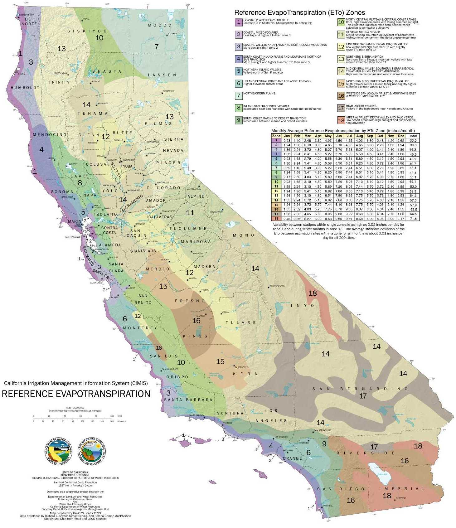
Create image file of Figure 3-12 Correlation Between Estimated Mean Annual Rainfall and Unit Streamflow for USGS Gaged Streams in the Santa Cruz Mountains Region for linkage here. Estimate regression line and add some discussion of that and local SC numbers.
Create image file of Figure 3-15 Correlation Between Annual Rainfall and Unit Streamflow Selected Periods of Gaged Record for linkage here.
Notice (quantify?) how much more streamflow varies than rainfall does.
Think about meaning of Big Trees panel of Figure 3-16 Estimated Avearge Stormflow-Baseflow Hydrograph Separation, Selected Gaged Streams
Would it make sense to add their Baseflow estimate to analysis above?
Create image file of Table 3-5 Periods of Above and Below Average Annual Rainfall, Selected Stations, WYs 1868-2006 for linkage here.
Add update for Santa Cruz 2009 to present to put current situation in better perspective.
Think about Table 3-10 Estimated Average Monthly Soil-Water Budgets
From earlier document.
The SLVWD Water Supply Master Plan May 2009 mentions three sources for long term monthly precipitation data and two for annual (back to the 1800s) precipitation data. Here is the description from the chapter 3 text
Table 3-1 summarizes information for selected rainfall stations in the region and Figure 3-1 shows their location.
Tables 3-2, 3-3, and 3-4 provide monthly rainfall records for three stations in the study area with relatively long records: the Santa Cruz and Ben Lomond 4 NOAA stations and the station near the crest of Ben Lomond Mountain now maintained by the nearby Lockheed facility. The available monthly records of these three stations extend back to 1931, 1973, and 1959, respectively. Table 3-5 provides annual rainfall totals for the Santa Cruz and Lockheed stations extending back to the 1800s.
Figure 3-1 includes an isohyetal (precipitation contours) map which is interesting.
7 City of Santa Cruz Water Meter Upgrade Project
This project is somewhat related to local water issues. The new water meters can be distinguished from outside the box by observing the circular black rubber portion (I believe that covers the antenna) on the meter boxes.
https://www.cityofsantacruz.com/government/city-departments/water/conservation/meter-replacement-project
https://utilitypartners.com/city-of-santa-cruz-selects-utility-partners-of-america-for-meter-replacement-project/
Excerpt from notification letter.
Starting in January 2022, we’ll be replacing most meters in the Santa Cruz Water Department service area. The whole project will take roughly 12 months to complete, and we’ll be replacing meters in your area about 4 to 6 weeks from the mailing date of this letter.
The detailed schedule is available at Meter Replacement Project Schedule. You can use your route number (first three digits of SCMU account number) to look up your notification dates and estimated install window.
8 So How Wet Is This Year?
After the background above I think the best way to answer this is to offer these plots (semi-duplicates from above) showing our relative status so far along with the current year compared with past full years to make clear just how much of the important part of the water year remains.
filter(flow.and.precip, wateryear > 2009) %>%
  filter(site_no == "11160500") %>%
  ggplot(aes(x = hydroday, y = wy_runoff_af, group = wateryear1, color = wateryear1)) +
  geom_line() +
  geom_dl(aes(label = wateryear1), method = "last.points", cex = 0.8) +
  geom_line(data = avg.runoffs[avg.runoffs$site_no == "11160500",]) +
  geom_hline(yintercept=c(48000, 29000), color=c('yellow', 'red')) + # Dry and critically dry levels
  labs(title = "Cumulative Water Year Runoff 2010 - 2022 at Big Trees",
       y = "Cumulative Runoff (acre-feet)",
       x = "Day of Water Year") +
  scale_y_continuous(labels = comma)
filter(flow.and.precip, wateryear > 2009) %>%
  ggplot(aes(x = hydroday, y = wy_PRCP, group = wateryear1, color = wateryear1)) +
  geom_line() +
  geom_dl(aes(label = wateryear1), method = "last.points", cex = 0.8) +
  geom_line(data = avg.PRCP[avg.PRCP$site_no == "11160500",]) +
  labs(title = "Cumulative Precipitation 2010 - 2022 at Santa Cruz",
       y = "Precipitation (inches)",
       x = "Day of Water Year")
So we can see over the last few weeks we have gone from an above average water year (for the date) to more of an average water year. But it is clearly too early to tell overall and the next 90 days are needed to make things clear.
Of course, water years should not just be considered in isolation. 2022 is notable for the two previous water years being among the driest of the last 85!
One way to look at this is to consider moving averages as done in Figure 3-8 from the SLVWD Water Supply Master Plan May 2009.

Figure 3-8 Minimum and Maximum Moving Average Rainfall
This could be extended to show the moving averages for the current year (or their trend over time). It is also possible to look at stream discharge in a similar fashion. Perhaps in another piece? (Science committee: or fold in above, it probably would not be THAT hard to do) It might also be interesting to show the distributions in addition to just the min/max. Perhaps something like a set of box plots for each moving average window?
9 Technical Notes
The Big Trees flow data above is not adjusted for diversions. See discussion in SLVWD Water Supply Master Plan May 2009. In particular, Table 3-13 contains the data they used, but I don’t have the knowledge or resources to make the same adjustments to the data above for more recent years (post 2008). They cite the “method of Geomatrix, 1999” but I have been unable to find further details.
Leap years are not handled well above. In particular, notice the downward glitch for the final day of the average cumulative precipitation and runoff plots.
10 File History
File Initially created: January, 24, 2022
File knitted: Tue Jan 25 21:15:17 2022