Pharmacometric Model Development

With R and NONMEM

1 R + Markdown = RMarkdown

1.1 R

is ‘GNU S’, a freely available language and environment for statistical computing and graphics which provides a wide variety of statistical and graphical techniques: linear and nonlinear modelling, statistical tests, time series analysis, classification, clustering, etc. Please consult the R project homepage for further information.

R can be executed from the command line and R scripts can be written in any text editor. However, the probably most efficient way to work with R (and related tools) is using the excellent R development environment RStudio. Details can be found at the RStudio homepage

R is a modular environment in a way that it consists of the well maintained R core system and a tremendous amount of R packages for all sorts of statistical (and other) aspects.

Statistical R packages include lme4 (linear mixed effects models), nlme (nonlinear mixed effects models), glm generalized linear models, survival (survival models) and many more.

Some of the most powerful non-statistical R packages are:

• tidyverse: data management
• ggplot2: plotting
• knitr and rmarkdown: report generation
• shiny: interactive applications
• plotly: interactive plots

1.2 Markdown

R Markdown is an easy-to-write plain text format for creating dynamic documents and reports. See Using R Markdown to learn more.

Text Formatting

*italic*   **bold**
_italic_   __bold__
superscript^2^
subscript~2~
~~strikethrough~~

For example: thinkQ².

Headers

# Header 1

## Header 2

### Header 3

Lists

Unordered List

* Item 1
* Item 2
    + Item 2a
    + Item 2b

• Item 1
• Item 2
  • Item 2a
  • Item 2b

Ordered List

1. Item 1
2. Item 2
3. Item 3
   + Item 3a
   + Item 3b

1. Item 1
2. Item 2
3. Item 3
   • Item 3a
   • Item 3b

Links

Use a plain http address or add a link to a phrase:

http://example.com

[linked phrase](http://example.com)

Click this link to see the thinkQ² homepage at https://www.thinkq2.com.

Images

Images on the web or local files in the same directory:

![alt text](http://example.com/logo.png)

![alt text](figures/img.png)

RStudio Icon

Blockquotes

A friend once said:

> It's always better to give 
> than to receive.

A friend once said:

It’s always better to give than to receive.

LaTeX Equations

Inline Equation

$N(\mu,\sigma)$ refers to a normal distribution with mean $\mu$ and standard deviation $\sigma$.

\(N(\mu,\sigma)\) refers to a normal distribution with mean \(\mu\) and standard deviation \(\sigma\).

Display Equation

$$
\sin(x) = \sum_{n=0}^{\infty} (-1)^n \frac{x^{2n+1}}{(2n+1)!}
$$

\[ \sin(x) = \sum_{n=0}^{\infty} (-1)^n \frac{x^{2n+1}}{(2n+1)!} \]

Horizontal Rule / Page Break

Three or more asterisks or dashes:

******

------

---

Tables

First Header  | Second Header
------------- | -------------
Content Cell  | Content Cell
Content Cell  | Content Cell

First Header	Second Header
Content Cell	Content Cell
Content Cell	Content Cell

and some more …

1.3 RMarkdown

Rmarkdown is a markdown extension to allow embedding R code in markdown documents.

R Code Blocks

R code will be evaluated and printed

```{r}
x <- rnorm(10, 0.0, 1)
y <- rnorm(10, .5, 1)
t.test(x, y)
```

    Welch Two Sample t-test

data:  x and y
t = -2.4821, df = 17.979, p-value = 0.02317
alternative hypothesis: true difference in means is not equal to 0
95 percent confidence interval:
 -1.696802 -0.141042
sample estimates:
 mean of x  mean of y 
-0.1329441  0.7859778 

Inline R Code

There were `r nrow(cars)` cars studied.

There were 50 cars studied.

NONMEM Control Blocks

Thus requires the MeRmd package (developed by myself and not yet open source)

```{NONMEM base-model}
$PK
  A = THETA(1) + ETA(1)

$PRED
  CONC = EXP(-A*TIME)

...
```

1.4 Report Generation

The knitr package extracts all R code blocks from an Rmd file, executes the contained R code and replaces the original code blocks with the generated output.

Any R code is allowed and entire statistical analyses can be executed within an RMarkdown document. Beside the reporting functionality, this also ensures a correct execution order of dependent steps.

There is also a caching mechanism which checks if code blocks require re-execution in case input variables have changed.

Output could be simple text (displayed as such) but also figures or tables. E.g. the following lines of R code in a code block would create the figure below:

set.seed(1234)

sample <- rnorm(100,5, 1) # 100 random numbers ~ N(5, 1)

hist(sample) # draw a simple histogram
abline(v = mean(sample), col = "orange", lwd = 2) # add the mean as vertical line

2 Pharmacometric Models

In contrast to bio-statistical model based analysis, pharmacometric analyses are typically not only dependent on the data but also on other sources of information (in form of assumptions and included/excluded mode features). The goal is to find a model that captures the relevant biology / pharmacology / physiology and is supported by the observed data.

Try to build a (semi-)mechanic model to characterize the relevant data features

• what is relevant / essential / a signal? (\(\rightarrow\) fixed effects)
• what is irrelevant / noise? (\(\rightarrow\) random effects)

The benefit of this approach is a hopefully better ability to make predictions at the cost of less rigorous point estimates. This is why pharmacometric models are rarely used for proofing (no hard test, p-values).

Typical elements of pharmacometric model based analyses

• understand the biology / pharmacology / physiology
• explore the data
• develop a semi-mechanistic model and fit parameters to the observed data
• ensure the the model represents the data
• use the model for what if scenarios

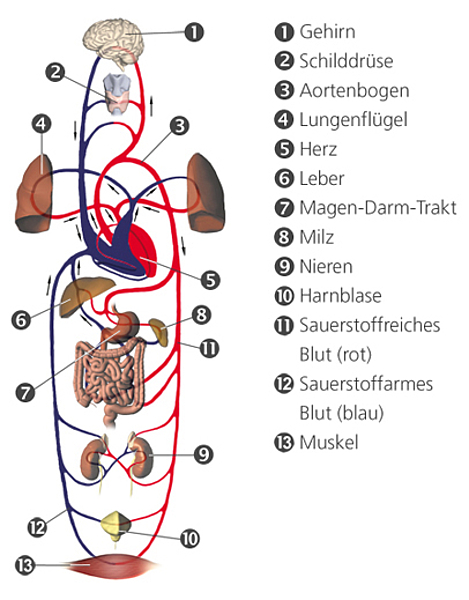
2.1 Biological Model

https://www.fosberlin.eu/fileadmin/_processed_/8/0/csm_blutkreislauf-frei-24-02-07_4e817f7c20.jpg

2.2 Abstract Model

2.3 Mathematical Model

The ODE for this model is given by \[ \begin{aligned} \frac{d}{dt} \textit{gut}(t) &= -k_\text{abs} \cdot \textit{gut}(t) \\ \frac{d}{dt} \textit{plasma}(t) &= k_\text{abs} \cdot \textit{gut}(t) - k_\text{el} \cdot \textit{plasma}(t) \\ &\quad- k_\text{2,3} \cdot \textit{plasma}(t) + k_\text{3,2} \cdot \textit{fat}(t) \\ \frac{d}{dt} \textit{fat}(t) &= +k_\text{2,3} \cdot \textit{plasma}(t) - k_\text{3,2} \cdot \textit{fat}(t) \end{aligned} \]

with initial condition (single dose at time 0): \[ \textit{gut}(0) = \textit{dose}. \]

Because we initialize zhis ODE with amounts (a dose in mg), all compartments will describe amounts (in mg) as well. In order to predict concentrations, we further need to estimate a volume parameter (V) (in L) and convert the outout into ng/mL (which is the usual unit for concentrations).

\[ \textit{conc}(t) = \textit{plasma}(t) / V / 1000 \] WARNING with intuitive parameter names …

2.3.1 Variables

• data variables need to be contained in the input dataset: \(\textit{dose}\) (AMT), \(\textit{conc}\) (DV), and \(\textit{t}\) (TIME)
• parameters will be estimated: \(k_\text{abs}\) (absorption rate KA), \(k_\text{el}\) (elimination rate KEL), \(k_{2,3}\)/\(k_{3,2}\) (distribution rates K23, K32), and \(\textit{V}\) (volume of distribution V). Because the structural model is nonlinear, starting values for the iterative estimation procedure are required.
• state variables will be obtained by solving the ODEs (using the data variables and parameters)

2.3.2 Dosing

Doses can be as simple as a single-dose bolus, i.e. just a starting value as used above. Other drug inputs might be cyclic (daily doses) and/or over a period of time (infusions, disturbed left-hand side).

2.4 Nonlinear Mixed Effects Models – Grouped Data

2.4.1 Single Group Case

Observations \(y_{i} = y(t_i)\) (DV) at times \(t_i\) (TIME). \(i\) denotes the observation number.

Model prediction \(f(t_i, \mathbf{p}, \mathbf{v})\) (obtained by solving the ODE using parameters \(\mathbf{p}\) and variables \(\mathbf{v}\))

\[ y_{i} = f(t_i, \mathbf{p}, \mathbf{v}) + \epsilon_i,\quad\text{where }\epsilon_i \sim N(0, \sigma^2). \]

2.4.2 Multiple Groups (e.g. Subjects)

Observations \(y_{i,j} = y_j(t_{i,j})\) at times \(t_{i,j}\). \(i\) denotes the observation number and \(j\) is the group (subject) number.

Model prediction \(f(t_{i,j}, \mathbf{p}_j, \mathbf{v}_j)\) using the individual parameters and variables.

\[ y_{i,j} = f(t_{i,j}, \mathbf{p}_j, \mathbf{v}_j) + \epsilon_i,\quad\text{where }\epsilon_i \sim N(0, \sigma^2). \]

\[ \mathbf{p}_j = \mathbf{p}^\text{typ} + \mathbf{\eta}_j\quad\text{where }\mathbf{\eta}_j \sim N(0, \Omega^2). \]

2.4.3 Other Grouping Levels

\[ \mathbf{p}_j = \mathbf{p}^\text{typ} + \mathbf{\eta}_j + \begin{cases} \mathbf{\kappa}^{(1)}_j & \text{if occasion 1} \\ \mathbf{\kappa}^{(2)}_j & \text{if occasion 2} \\ \ldots & \end{cases} \]

2.5 Covariate Analysis

We typically do not pre-define covariates but try to screen for significant and relevant covariates during model development. We think of covariates a variables helping to explain variability. Covariates should improve the fit, reduce the variability, reduce variable-parameter correlations, resolve bi-(or multi-)modal random effect distributions.

\[ \begin{aligned} p^\text{typ} &= \theta_1 &\quad\text{typical value}\\ p^\text{typ} &= p^\text{typ} \cdot \left(\frac{\textit{weight}}{70}\right)^{\theta_2} &\quad\text{weight effect, power model}\\ p^\text{typ} &= p^\text{typ} \cdot (1 + (\textit{age}-40)\cdot\theta_3) &\quad\text{age effect, linear model}\\ p^\text{typ} &= p^\text{typ} \cdot (1 + 1_{\textit{sex}=\text{Female}}\cdot\theta_4/100) &\quad\text{gender effect, percent}\\ p^\text{typ} &= p^\text{typ} + 1_{\textit{race}=\text{Asian}}\cdot\theta_5 &\quad\text{Asian effect, absolut}\\ \end{aligned} \]

2.6 (Non-Normal) Error Models

By default, NONMEM (and probably most model fitting tools) provide only normal distributed random effects. Random effects always have a mean of 0 (typical deviations must be estimated as fixed effects) and a variance which will be estimated. There are two types of random effects:

• OMEGA: subject level random effects (which can also be used for other grouping levels)
• SIGMA: observation level random effects

Non-normal variability models are used by transforming the normal random effect variables. Let \(\eta\) be a normal distributed random effect with mean 0 and variance \(\omega^2\).

\[ \begin{aligned} p &= p^\text{typ} + \eta &\quad\text{Normal}\\ p &= p^\text{typ} \cdot e^\eta &\quad\text{LogNormal}\\ p &= p^\text{typ} \cdot \frac{e^\eta}{1+e^\eta} &\quad\text{Logit}\\ p &= p^\text{typ} \cdot \text{BoxCox}(\eta, \textit{shape}) &\quad\text{custom, e.g. Box-Cox transformed} \end{aligned} \]

3 Model Types

Most frequently, models are used to characterize the PK but also PD (biomarker and efficacy endpoints) as well as safety readouts are modeled.

This requires a wide spectrum of pharmacometric model types

• PK models
  • most frequently compartmental ADME models
  • linear PK:
    • 1-, 2-, 3- compartment models
    • with or without absorption
  • non-linear PK
    • Michaelis Menten
    • target-mediated drug disposition
• PK/PD models
  • for continuous PD
    • direct link: linear, Emax
    • indirect link: turnover models, endogenous feedback
  • count models: binomial, Poisson, neg-bin, …
  • event data: survival, TTE, RTTE
  • (pain-) scores: state models (e.g. HMM)

Sometimes even more complex models are used, e.g. when the PD effect has a feedback loop on PK.

4 NONMEM

NONMEM is a quite generic software (written in FORTRAN 95) to fit almost any type of nonlinear mixed effects model to data. It is very flexible in terms of the model definition. There is no gui. NONMEM is controlled by using so called control-streams which define the data, the model, as well as all other configuration options.

4.1 Control Streams

A NONMEM control stream is a text file structured in different sections as described below. The data is not defined in the control stream but kept in a separate file which is refreenced by the control stream.

4.1.1 Structural Model ($DES, $PRED, $SUBROUTINE)

The structural model connects the biological/medical understanding with the data

• often, so called compartmental models are used to describe the mass transfer using ODEs
• parameters are used to quantify rates, volumes, delay times, …

Most often, the structural model is defined using differential equations. In this case, the control streams needs a section $DES (differential equations).

State variables are called A(1), A(2), … (because they typically describe amounts).

The 2-Compartment ODE from above would be written as

$DES
  DADT(1) = -KA*A(1)
  DADT(2) =  KA*A(1) -KEL*A(2) -K23*A(2) + K32*A(3)
  DADT(3) =                     K23*A(2) - K32*A(3)

Standard models are pre-defined (and also use closed form solutions instead of ODE solvers). Such predefined structural models are chosen in the $SUBROUTINE section.

$SUBROUTINE ADVAN4 TRANS4

In case the model is defined using algebraic equations (instead of ODEs), the $PRED section needs to be used.

$PRED
  EFF = E0 + EMAX * CONC / (EC50 + CONC)

4.1.2 Parameter Models ($PK)

The model parameters (parameter models, i.e. fixed and random effects) are defined in the $PK control stream section. E.g. the KA parameter could be modeled as

$PK
  TVKA = THETA(1)
  TVKA = TVKA * (WEIGHT/70)**THETA(2)
  IF( SEX==2 ) TVKA = TVKA * (1 + THETA(3)/100)
  ...
  KA = TVKA * EXP(ETA(1))

4.1.3 Starting Values ($THETA, $OMEGA, $SIGMA)

4.1.4 Residual Error Models ($ERROR)

Like parameter variability models, residual variability models are also frequently transformed Normal random effects. The example below shows a residual error term which is factored into an additive and a proportional component.

Frequently, the estimated standard deviation of the residual error is also used for weighing residuals. When the parameter estimation is based on maximum likelihood, the objective function (similar to the sum of squares of the weighted residuals) gets minimized. Therefore, weights can be used to selectively focus on certain samples.

$ERROR
  IPRED = A(2)/V                                ; ind. prediction
  SD = SQRT(THETA(1)**2 + (IPRED*THETA(2))**2)  ; std.dev. of RUV
  
  IRES = IPRED-DV                               ; ind. residual
  IWRES = IRES * 1/SD                           ; ind. weighted residual
  
  Y = IPRED + SD*SIGMA(1)                       ; ind. pred. with N(0, SD)

In addition to the above defined individual results (IPRED, IRES, IWRES), NONMEM also calculates population results (PRED, RES, WRES) by internally setting all ETAs to 0.

4.2 Parameter Estimation ($ESTIMATION, $COVARIANCE)

By default, NONMEM uses a maximum likelihood approach to estimate all fixed and random effect parameters. Numerically, this is similar to minimizing the objective function which is proportional to -2LL (\(-2\cdot\text{log}(\text{likelyhood})\)). This in turn is similar to the sum of squares of the weighted residuals which is defined using the observations and the model predictions which are a function of the model parameters.

Therefore, a gradient method can be used to minimize this function based on the partial derivatives with respect to the model parameters.

4.3 Simulations ($SIMULATE)

Once, the parameters are estimated, NONMEM can also be used to simulate the model response. A dataset needs to be created defining the data variables (subject characteristics, treatments, etc.) and the sampling times. NONMEM will calculate the population parameters (fixed effects only) and use random number generators to simulate individual parameters. Those will be used to calculate model predictions at the specified sampling times.

More about this in the Simulations section below.

4.4 Data ($DATA, $INPUT)

The analysis dataset + needs to contain all input and output of the system to be described. + e.g. for a PK model, the data needs to contain - dosing events (when, how much, how) - PK samples (time and concentrations) - patient characteristics (anything which might affect the ADME) - study structure (to define grouping levels) + mandatory variables for NONMEM are - grouping and time: ID, TIME, EVID (+ PERIOD, SEQUENCE, \(\ldots\)) - dosing: AMT, (+ FORMULATION, CMT, \(\ldots\)) - PK concentrations: DV, (+ DVID, \(\ldots\)) - other: WEIGHT, SEX, AGE

4.5 Final Silexan Model

4.5.1 Dataset

Special NONMEM columns:

• ID: used for grouping
• TIME: time for dosing and observations
• EVID: event ID: 0 = output (PK conc.), 1 = input (dose)
• AMT: dosing amount
• DV: dependent variable (PK conc)

NONMEM data needs to be purely numeric, i.e. text-variables need to be encoded as numbers:

Potential missing values were converted as NA.

• STUDY: ‘750201.01.023’->1, ‘750201.01.024a’->2, ‘750201.01.024b’->3, ‘750201.01.024c’->4
• FORM: ‘standard softgel capsule’->1, ‘delayed release softgel capsule’->2
• BLQ: converted with as.logical()
• SEX: ‘Male’->1, ‘Female’->2

4.5.2 Control Stream

5 Model Assements

5.1 Numerical Results

5.1.1 Parameter Estimates and Precision

The model turned out to be too complex and the calculation of standard errors failed. A bootstrap procedure could have been performed instead (but was not done as the parameters itself were not of major interest).

Other numerical results:

• convergence properties
• parameter correlations
• shrinkage

5.2 Residual-Based Diagnostics

5.2.1 Observation-Level

Observations vs. Predictions

Check overall alignment (close to diagonal).

Distribution of Residuals

Check normality (no bias, symmetric, quantiles).

Distribution vs. Time After Dose

Check for trends over time (mean and variability). Tells about temporal model mis-specifications.

Distribution vs. (Predicted) Concentrations

Check for trends over conc (mean and variability). Tells about issues with particular concentration ranges (e.g. C_max)

5.2.2 Subject-Level

\(\eta\)-Distributions

5.3 Simulation Based Diagnostics

These assesments are typically the most important. Only if the model predictions reliably match with the observations, the model can be used instead of the data.

6 Simulations and Predictions

6.1 NCA-Style (Individual Estimates)

In this case, the individual parameter estimates are used to predict (calculate with out random number generators) very dense individual profiles. These profiles are then used to calculate NCA-like parameters like AUC, C_max, etc.

6.2 Full Simulations

Here, individual parameters are simulated using a random number generator to sample from the random effect distributions. Typically three levels of results are generated:

• PRED: typical parameters (and hence PK profile) for a subject with these characteristics (deterministic, \(\eta=0\) and \(\epsilon=0\))
• IPRED: random parameters (and hence PK profile) for a subject with these characteristics (simulation, \(\eta \sim N(0, \omega^2)\) and \(\epsilon=0\))
• DV: additionally with residual error (simulation, \(\eta \sim N(0, \omega^2)\) and \(\epsilon \sim N(0, \sigma^2)\))

7 Clinical Trial Simulations

Typically, the PK or PK/PD model only captures certain aspects of a future study outcome. For a proper clinical trial simulation, other sources of variability should be considered.

• population variability
  • given the (draft) study protocol, what subjects will be likely included in the study population?
  • how can (correlated) subject characteristics be generated?
• dropout variability
  • do we have dropout?
  • is this purely at random?
  • how can we mimic a realistic dropout?
• compliance variability
  • can we expect full compliance?
  • how can we mimic a compliance pattern?

Typical steps of a CTS

1. Study Setup
   • Genarate a plausible study population (covariates)
   • Generate the study structure (periods, visits, optionally with dropout)
   • Generate treatment events and sampling times
2. Study Execution
   • Use the PK model to simulate the PK
   • Use the PK/PD model to simulate PD
   • apply dropout model (if not random)
3. Evaluate the Study
   • derive results (e.g. NCA, change from baseline, …)
   • perform the planned statistical tests (e.g. BE statistics on AUC and Cmax)
4. Repeat 1 – 3 many times and summarise results