Week of November 15
sileshi boru
library(tidyverse)## ── Attaching packages ─────────────────────────────────────── tidyverse 1.3.1 ──## ✓ ggplot2 3.3.5 ✓ purrr 0.3.4
## ✓ tibble 3.1.6 ✓ dplyr 1.0.7
## ✓ tidyr 1.1.4 ✓ stringr 1.4.0
## ✓ readr 2.1.0 ✓ forcats 0.5.1## ── Conflicts ────────────────────────────────────────── tidyverse_conflicts() ──
## x dplyr::filter() masks stats::filter()
## x dplyr::lag() masks stats::lag()library(nycflights13)Working with Relational Data
So far you have been working with data in one table. Usually stored as a tibble or a dataframe. But IRL (and even the the Metaverse :)) it is a rare thing to work with only one table. Most frequently this takes the froms of working with a relational base. And while there exist specialized languages, most notably SQL, to work with relational data bases, it is useful to be able to perform some of the same functions in your development language, whether that be R, Pyton, Julia, Matlap, Tableau, even Excel.
Last week you worked with the nycflights13 data base, but you worked only with the flights table. I believe I mentioned the fact that nycflights13 had other tables as well.
Task 1
Since this is a new project, you will have to install both
nycflights13andtidyverse. Useinstall.packagesbut do the installation in the console pane. library(nycflights13)Load these packages in the first code chunck of this project.
Use the help system to answer the following questions:
- How mamny tables are there in the databas
b. How many airports are represented in the table?
Your answer:1458
c. What are the variables in planes table?
Your answer:
## Introduction to relational data
*You will find Chapter 13 in [R for Data Science](https://r4ds.had.co.nz/relational-data.html#relational-data) usefull background reading.*
The following passage is from R4DS:
"To work with relational data you need verbs that work with pairs of tables. There are three families of verbs designed to work with relational data:
* **Mutating joins**, which add new variables to one data frame from matching observations in another.
* **Filtering joins**, which filter observations from one data frame base
* **Set operations**, which treat observations as if they were set elements.
The most common place to find relational data is in a relational database management system (or RDBMS), a term that encompasses almost all modern databases. If you’ve used a database before, you’ve almost certainly used SQL. If so, you should find the concepts in this chapter familiar, although their expression in dplyr is a little different. Generally, dplyr is a little easier to use than SQL because dplyr is specialised to do data analysis: it makes common data analysis operations easier, at the expense of making it more difficult to do other things that aren’t commonly needed for data analysis.d on whether or not they match an observation in the other table.
### Task 2
Examine the following table and verify that the associations depicted between the data tables is correct. (also from R4DS)
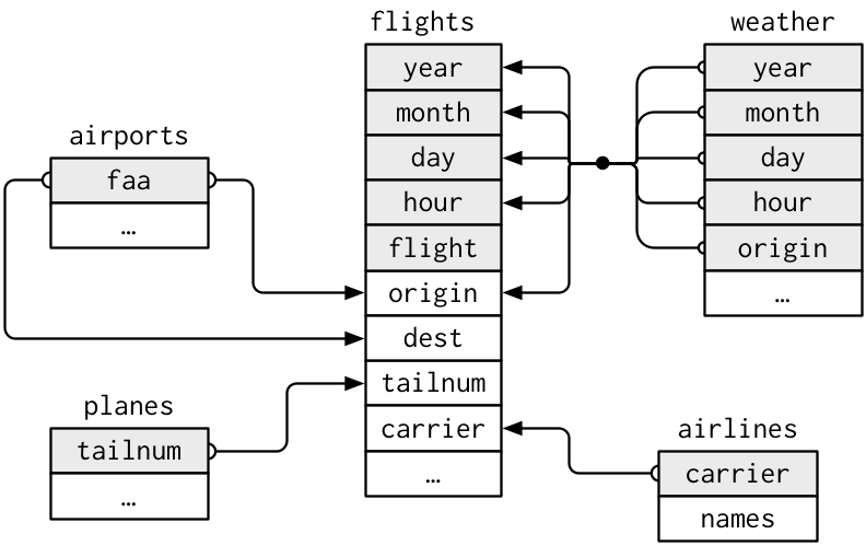
1. What information can be gained that would not be in the flights data table? (be specific)
2. Suppose you wanted to approximate the route each plane flies from its origin to its destination. What variables would you need? What tables would you need to combine?
3. There is connection between `weather` and `airports`, not shown in the figure above. What is the relationship and how would it appear?
4. `weather` only contains information for the origin (NYC) airports. If it contained weather records for all airports in the USA, what additional relation would it define with `flights`?
---
Connecting variables are called **keys**. By definition a key is a variable or set of variables that uniquely identifies an observation.
#### Types of keys
1. **primary key** uniquely identifies an observation in its own table.
2. **foreign key** uniquely identifies an observation in another table.
**Definition:** A primary key and a matching foreign key in another table define a **relation**.
---
### Taks 3
1. A variable can be both a primary and foreign key? Can you give an example from `nycflights13`?
2. How can you verify that a key is a primary key? (Hint, you will probably need to write some code!)
3. What is the primary key for `flights`?
---
If a table does not have a primary key then if a primary key is needed, then one can be created using `mutate`() and `row_number`(), such a created key is called a **surrogate key**.
---
### Task 4
1. Are relations one-to-one or one-to-many?
2. Can there be a many-to-many relations?
3. What variables would you use to create a surrogate key for `flights`?
4. Identify the keys in the following datasets:
* `Lahman::Batting`
* `babynames::babynames`
* `nasaweather::atmos`
* `fueleconomy::vehicles`
* `ggplot2::diamonds`
---
## Mutating joins
A **mutating join** allows you to combine variables from two tables.
Example:
```r
flights2 <- flights %>%
select(year:day, hour, origin, dest, tailnum, carrier)
flights2## # A tibble: 336,776 × 8
## year month day hour origin dest tailnum carrier
## <int> <int> <int> <dbl> <chr> <chr> <chr> <chr>
## 1 2013 1 1 5 EWR IAH N14228 UA
## 2 2013 1 1 5 LGA IAH N24211 UA
## 3 2013 1 1 5 JFK MIA N619AA AA
## 4 2013 1 1 5 JFK BQN N804JB B6
## 5 2013 1 1 6 LGA ATL N668DN DL
## 6 2013 1 1 5 EWR ORD N39463 UA
## 7 2013 1 1 6 EWR FLL N516JB B6
## 8 2013 1 1 6 LGA IAD N829AS EV
## 9 2013 1 1 6 JFK MCO N593JB B6
## 10 2013 1 1 6 LGA ORD N3ALAA AA
## # … with 336,766 more rowsSuppose you wand to add the full airline name to the flights2 data.
You can combine airlines and flights2 data frames with left_join()
flights2 %>%
  select(-origin,-dest) %>%
  left_join(airlines,by = "carrier")
## # A tibble: 336,776 × 7
## year month day hour tailnum carrier name
## <int> <int> <int> <dbl> <chr> <chr> <chr>
## 1 2013 1 1 5 N14228 UA United Air Lines Inc.
## 2 2013 1 1 5 N24211 UA United Air Lines Inc.
## 3 2013 1 1 5 N619AA AA American Airlines Inc.
## 4 2013 1 1 5 N804JB B6 JetBlue Airways
## 5 2013 1 1 6 N668DN DL Delta Air Lines Inc.
## 6 2013 1 1 5 N39463 UA United Air Lines Inc.
## 7 2013 1 1 6 N516JB B6 JetBlue Airways
## 8 2013 1 1 6 N829AS EV ExpressJet Airlines Inc.
## 9 2013 1 1 6 N593JB B6 JetBlue Airways
## 10 2013 1 1 6 N3ALAA AA American Airlines Inc.
## # … with 336,766 more rowsUnderstanding joins
Consider the data frames:  We can make this data as follows:
x <- tribble(
  ~key, ~val_x,
     1, "x1",
     2, "x2",
     3, "x3"
)
y <- tribble(
  ~key, ~val_y,
     1, "y1",
     2, "y2",
     4, "y3"
)
x
## # A tibble: 3 × 2
## key val_x
## <dbl> <chr>
## 1 1 x1
## 2 2 x2
## 3 3 x3y## # A tibble: 3 × 2
## key val_y
## <dbl> <chr>
## 1 1 y1
## 2 2 y2
## 3 4 y3
 This type of join is called an inner join which means pairs of observations are matched when their keys are equal.
x %>%
  inner_join(y, by = "key")
## # A tibble: 2 × 3
## key val_x val_y
## <dbl> <chr> <chr>
## 1 1 x1 y1
## 2 2 x2 y2#> # A tibble: 2 x 3
#> key val_x val_y
#> <dbl> <chr> <chr>
#> 1 1 x1 y1
#> 2 2 x2 y2notice: unmatched rows are not included in the result.
Outer Joins
While an inner join keeps only observations that appear in both tables and outer join keeps all observations that appear in one of the tables.


What Happens when we have duplicate keys
All the diagrams above assume that there are no duplicate keys in a data set. Is this even true for flights? Can you think of an example?
Here is a diagram from Wickham and Grolemund illustrating the situation

x <- tribble(
  ~key, ~val_x,
     1, "x1",
     2, "x2",
     2, "x3",
     1, "x4"
)
y <- tribble(
  ~key, ~val_y,
     1, "y1",
     2, "y2"
)
left_join(x, y, by = "key")
## # A tibble: 4 × 3
## key val_x val_y
## <dbl> <chr> <chr>
## 1 1 x1 y1
## 2 2 x2 y2
## 3 2 x3 y2
## 4 1 x4 y1#> # A tibble: 4 x 3
#> key val_x val_y
#> <dbl> <chr> <chr>
#> 1 1 x1 y1
#> 2 2 x2 y2
#> 3 2 x3 y2
#> 4 1 x4 y1Note: in this case, key is a foreign key in x and a primary key in y.
If boh tables have duplicate keys the keys do not uniquely identify an observation. In this case a join results in all possible combinations (cartesian product)

x <- tribble(
  ~key, ~val_x,
     1, "x1",
     2, "x2",
     2, "x3",
     3, "x4"
)
y <- tribble(
  ~key, ~val_y,
     1, "y1",
     2, "y2",
     2, "y3",
     3, "y4"
)
left_join(x, y, by = "key")
## # A tibble: 6 × 3
## key val_x val_y
## <dbl> <chr> <chr>
## 1 1 x1 y1
## 2 2 x2 y2
## 3 2 x2 y3
## 4 2 x3 y2
## 5 2 x3 y3
## 6 3 x4 y4Defining Key Columns
In the above examples the key values were single variables and in left_jointhe ke was encoded by by = "key". But one can use other values for by= the default is by = NULL. What does this mean?
#let's get flights2 back to eliminate extraneous columns
flights2 <- flights %>%
  select(year:day, hour, origin, dest, tailnum, carrier)

flights2 %>%
  left_join(weather) #note I'm taking all the defaults
## Joining, by = c("year", "month", "day", "hour", "origin")## # A tibble: 336,776 × 18
## year month day hour origin dest tailnum carrier temp dewp humid
## <int> <int> <int> <dbl> <chr> <chr> <chr> <chr> <dbl> <dbl> <dbl>
## 1 2013 1 1 5 EWR IAH N14228 UA 39.0 28.0 64.4
## 2 2013 1 1 5 LGA IAH N24211 UA 39.9 25.0 54.8
## 3 2013 1 1 5 JFK MIA N619AA AA 39.0 27.0 61.6
## 4 2013 1 1 5 JFK BQN N804JB B6 39.0 27.0 61.6
## 5 2013 1 1 6 LGA ATL N668DN DL 39.9 25.0 54.8
## 6 2013 1 1 5 EWR ORD N39463 UA 39.0 28.0 64.4
## 7 2013 1 1 6 EWR FLL N516JB B6 37.9 28.0 67.2
## 8 2013 1 1 6 LGA IAD N829AS EV 39.9 25.0 54.8
## 9 2013 1 1 6 JFK MCO N593JB B6 37.9 27.0 64.3
## 10 2013 1 1 6 LGA ORD N3ALAA AA 39.9 25.0 54.8
## # … with 336,766 more rows, and 7 more variables: wind_dir <dbl>,
## # wind_speed <dbl>, wind_gust <dbl>, precip <dbl>, pressure <dbl>,
## # visib <dbl>, time_hour <dttm>It means that we join by mathcing on all common variables, see console message above.
On the other hand if match on a key, for example tailnum is a foreign key in flights for planes
flights2 %>%
  left_join(planes, by="tailnum")
## # A tibble: 336,776 × 16
## year.x month day hour origin dest tailnum carrier year.y type
## <int> <int> <int> <dbl> <chr> <chr> <chr> <chr> <int> <chr>
## 1 2013 1 1 5 EWR IAH N14228 UA 1999 Fixed wing mult…
## 2 2013 1 1 5 LGA IAH N24211 UA 1998 Fixed wing mult…
## 3 2013 1 1 5 JFK MIA N619AA AA 1990 Fixed wing mult…
## 4 2013 1 1 5 JFK BQN N804JB B6 2012 Fixed wing mult…
## 5 2013 1 1 6 LGA ATL N668DN DL 1991 Fixed wing mult…
## 6 2013 1 1 5 EWR ORD N39463 UA 2012 Fixed wing mult…
## 7 2013 1 1 6 EWR FLL N516JB B6 2000 Fixed wing mult…
## 8 2013 1 1 6 LGA IAD N829AS EV 1998 Fixed wing mult…
## 9 2013 1 1 6 JFK MCO N593JB B6 2004 Fixed wing mult…
## 10 2013 1 1 6 LGA ORD N3ALAA AA NA <NA>
## # … with 336,766 more rows, and 6 more variables: manufacturer <chr>,
## # model <chr>, engines <int>, seats <int>, speed <int>, engine <chr>suppose we wanted to draw a map of all destination air ports for flights from NewYork in 2013
flights2%>%
  left_join(airports, c("dest"="faa"))
## # A tibble: 336,776 × 15
## year month day hour origin dest tailnum carrier name lat lon alt
## <int> <int> <int> <dbl> <chr> <chr> <chr> <chr> <chr> <dbl> <dbl> <dbl>
## 1 2013 1 1 5 EWR IAH N14228 UA Georg… 30.0 -95.3 97
## 2 2013 1 1 5 LGA IAH N24211 UA Georg… 30.0 -95.3 97
## 3 2013 1 1 5 JFK MIA N619AA AA Miami… 25.8 -80.3 8
## 4 2013 1 1 5 JFK BQN N804JB B6 <NA> NA NA NA
## 5 2013 1 1 6 LGA ATL N668DN DL Harts… 33.6 -84.4 1026
## 6 2013 1 1 5 EWR ORD N39463 UA Chica… 42.0 -87.9 668
## 7 2013 1 1 6 EWR FLL N516JB B6 Fort … 26.1 -80.2 9
## 8 2013 1 1 6 LGA IAD N829AS EV Washi… 38.9 -77.5 313
## 9 2013 1 1 6 JFK MCO N593JB B6 Orlan… 28.4 -81.3 96
## 10 2013 1 1 6 LGA ORD N3ALAA AA Chica… 42.0 -87.9 668
## # … with 336,766 more rows, and 3 more variables: tz <dbl>, dst <chr>,
## # tzone <chr>##Task 5 Homework - Exercises from 13.3.6
This work is based on “R for Data Science” by Hadley and Grolemund. Tt is licensed under
This work is licensed under the Creative Commons Attribution-NonCommercial-NoDerivs 3.0 United States License. To view a copy of this license, visit http://creativecommons.org/licenses/by-nc-nd/3.0/us/ or send a letter to Creative Commons, 444 Castro Street, Suite 900, Mountain View, California, 94041, USA.