如果想要深入了解这项技术，可以重点看看这本书：

推荐一下我自己写的书籍：

深入浅出R语言数据分析

R语言数据可视化实战

推荐一下我开发的IOS 增强现实软件：

敏捷数据科学

在介绍信用评分模型开发之前，我们来接单介绍一下方法论方面的东西。我们都知道，数据挖掘有很多方法论，包括业务理解，数据准备，数据分析特征选择，构建模型，模型评估等步骤。

比较著名的方法论是，CRISP-DM，全称为：Cross-Industry Standard Process for Data Mining，也就是跨行业的数据挖掘标准流，是SPSS公司1999年提炼出来的数据挖掘项目实践的标准方法论。

我们这里要讨论的方法论是比这个方法论还要高一个层级。我们要了解什么是敏捷数据科学，我们首先还是要了解什么是敏捷开发。

要了解敏捷（Agile）开发，首先需要了解的是软件开发的另外一个框架，waterfull。在 Waterfall 中，大型软件项目被划分为特定的阶段，每个阶段都应该完成，然后才能开始下一阶段。随后的这些阶段是问题分析、设计项目、编写软件、测试，最后是实施和维护。

Waterfall 的目标是提供完整且无故障的软件。Waterfall 项目的重中之重是文档，其中详细记录了软件的每个要求和方面。潜在的信念是，当软件的所有方面都预先决定时，它的编写速度更快，质量更高。但是waterfall 方法论太笨重了。waterfall方法完成的项目有一个主要的缺陷是项目需要很长时间才能完成。顺序性和完整性的结合可能会导致项目在交付软件之前持续多年。每次在后期阶段中发现错误或不完整时，项目就会返回上一阶段进行修复。由于整个过程持续时间长，经常出现最终结果不再适合不断变化的市场的情况。

基于waterfall 的缺陷，就有人提出了敏捷开发，关于敏捷开发，可以讲的内容有很多，但是总结而言是：快速交付最小可行性产品（MVP），然后不断迭代产品。

在数据科学中，据我所知，没有这样正式和广泛的方法论，我们可以借用敏捷开发的思想，敏捷数据科学指的是：快速交付最小可行性模型（MVM），然后不断迭代模型。

也就是说，不要无休止的探索数据，无休止的探索模型，优化参数，使用你能够拿得到的数据，使用你擅长的方法，尽快的交付一个可行性模型，让利益相关者、同事和客户在每个阶段都密切参与，然后不断的迭代模型。

相关书籍： ()[https://edwinth.github.io/ADSwR/]

评分卡开发流程

评分卡

标准评分卡

信用评分卡主要分为两类：

申请评分卡
行为评分卡

两种评分卡开发过程都是基于同样的方案，但是两者所应用的场景是有所不同的：

申请评分卡被用于对新贷款申请进行一次性的信用评分，来决定是否贷款，贷款额度，贷款定价行为评分卡是对于通过审批进入执行阶段的用户，即进行一定交易的用户，进行信用评分，结果用于制定清收策略

正常与违约

正常和违约通常不存在唯一的标准，其判定的标准往往取决于企业。但是，大多数评分卡开发都是基于60天，90天或者180天预期为标准。举个例子，标准可以定位，如果一个用户贷款逾期60天以上了，此时，定义这个用户为坏客户。

在运营商领域，我们构建流失模型的时候也需要定义什么是流失，通常而言，流失可以定义为，用户T月出账，T+1月不出账。

这个过程相当于打标签，如何打标签取决于具体的业务问题。

明确了正常和违约的含义之后，需要对数据进行打标签，通常使用1表示违约，0表示正常

标准评分卡的格式

当我们有了数据之后，就可以通过这个这个打分表来进行打分。

信用评分卡的优点

易于理解
总的分值由于每一个变量的分值组合而成，非常易于解释
简单，非常用以实现
用户可以非常清楚的知道自己如何提高自己的分数

评分卡开发流程

评分卡的开发流程大致如何，其实任何一个数据挖掘项目的开发流程都由类似的开发过程：

这个过程其实和数据挖掘的流程基本上是一致的。

数据准备

实际中，数据可能分散在各个地方，这个时候就需要将我们能够使用的所有的数据整合汇总起来。这一步其实不容易的，有什么数据可以用，什么数据合适用，什么数据有用，这些也许需要很多次尝试才能知道结果。

探索性分析

探索性分析是检查数据以及理解数据的一个过程，一般情况下，需要进行如下的一些分析：

特征的统计描述，取值范围
特征的违约率的分布（这一步需要对连续变量进行分箱）
通过卡方检验，相关性指标确定不同变量之间的关系

特征选择

如果有成百上千的建模特征，这个时候需要筛选出那些有非常好预测能力的并且有比较好解释性的变量。特征选择的方法有很多，评分卡最常用的特征选择方法就是使用IV值进行筛选，建立罗辑回归模型之后使用逐步回归进一步筛选特征。当然，还有很多机器学习的特征选择方法，比如随即森林，boruta等等

模型开发

构建模型，例如逻辑回归模型

模型验证

模型验证一般要保证四个基本要求

有比较好的准确度
模型应该稳健
模型必须简单
要有比较好的可解释性

分卡开发

当我们建立好罗辑回归模型之后，我们需要将罗辑回归的结果转变成为评分卡的形式，具体方法会在后面讲解

模型的上线与监控

评分卡建立好了之后，需要转化成为可以实施的代码，并且确定得分的临界值，以对应所需要的业务行动。

上线好之后需要监控，应为评分卡的应用环境是在不断变化的。因此必须监控评分卡的实际表现如何，评分卡的客户群的特征变化等等

数据获取与数据整合

信用评分卡的数据来源

一般而言，信用评分卡的数据主要可以分为如下几组：

人口统计特征，这个使用户的基本信息，包括，家庭收入，性别，年龄等
征信机构的数据，比如人行征信
交易数据，这一部分就很多的，购物信息，金融交易信息等等
其他产品所有权和使用记录，客户可能会在其他的金融机构同样有使用产品

在运营商这个行业，数据大致包含基本特征，产品特征，业务特征，消费特征，终端偏好等等。

有的时候，用户会有多条记录，因此需要用汇总值来处理，将多条记录转变成为1条记录.

汇总值有几类，这里可以做一个总结：

计数，有过多少次贷款，有过多少消费记录
求和，总的消费金额
占比，贷款额度与年收入的占比
时间差，第一次开户距今时常
波动率，过去三年每一份工作的时常标准差

完整性检验

数据获取并且整合之后，需要进行一些列完整性检验，包括

行的唯一性，一个ID只能有一条记录
范围与取值，每一个特征都需要有一个清晰的取值范围
缺失值，
样本是否能够代替整体

探索性分析

探索性分析需要做如下一些事情：

特征的统计描述以及分布
特征与预测变量之间的关系，特征是否有预测效果
缺失值与极端值的处理
特征中好坏样本的分布

这里使用scorecard包中的一份信用评分数据作为例子

library(scorecard)
data("germancredit")
names(germancredit)

##  [1] "status.of.existing.checking.account"                     
##  [2] "duration.in.month"                                       
##  [3] "credit.history"                                          
##  [4] "purpose"                                                 
##  [5] "credit.amount"                                           
##  [6] "savings.account.and.bonds"                               
##  [7] "present.employment.since"                                
##  [8] "installment.rate.in.percentage.of.disposable.income"     
##  [9] "personal.status.and.sex"                                 
## [10] "other.debtors.or.guarantors"                             
## [11] "present.residence.since"                                 
## [12] "property"                                                
## [13] "age.in.years"                                            
## [14] "other.installment.plans"                                 
## [15] "housing"                                                 
## [16] "number.of.existing.credits.at.this.bank"                 
## [17] "job"                                                     
## [18] "number.of.people.being.liable.to.provide.maintenance.for"
## [19] "telephone"                                               
## [20] "foreign.worker"                                          
## [21] "creditability"

summary(germancredit)

##                                      status.of.existing.checking.account
##  ... < 0 DM                                            :274             
##  0 <= ... < 200 DM                                     :269             
##  ... >= 200 DM / salary assignments for at least 1 year: 63             
##  no checking account                                   :394             
##                                                                         
##                                                                         
##  duration.in.month
##  Min.   : 4.0     
##  1st Qu.:12.0     
##  Median :18.0     
##  Mean   :20.9     
##  3rd Qu.:24.0     
##  Max.   :72.0     
##                                                      credit.history
##  no credits taken/ all credits paid back duly               : 40   
##  all credits at this bank paid back duly                    : 49   
##  existing credits paid back duly till now                   :530   
##  delay in paying off in the past                            : 88   
##  critical account/ other credits existing (not at this bank):293   
##                                                                    
##    purpose          credit.amount                 savings.account.and.bonds
##  Length:1000        Min.   :  250   ... < 100 DM               :603        
##  Class :character   1st Qu.: 1366   100 <= ... < 500 DM        :103        
##  Mode  :character   Median : 2320   500 <= ... < 1000 DM       : 63        
##                     Mean   : 3271   ... >= 1000 DM             : 48        
##                     3rd Qu.: 3972   unknown/ no savings account:183        
##                     Max.   :18424                                          
##        present.employment.since
##  unemployed        : 62        
##  ... < 1 year      :172        
##  1 <= ... < 4 years:339        
##  4 <= ... < 7 years:174        
##  ... >= 7 years    :253        
##                                
##  installment.rate.in.percentage.of.disposable.income
##  Min.   :1.000                                      
##  1st Qu.:2.000                                      
##  Median :3.000                                      
##  Mean   :2.973                                      
##  3rd Qu.:4.000                                      
##  Max.   :4.000                                      
##                         personal.status.and.sex other.debtors.or.guarantors
##  male : divorced/separated          : 50        none        :907           
##  female : divorced/separated/married:310        co-applicant: 41           
##  male : single                      :548        guarantor   : 52           
##  male : married/widowed             : 92                                   
##  female : single                    :  0                                   
##                                                                            
##  present.residence.since
##  Min.   :1.000          
##  1st Qu.:2.000          
##  Median :3.000          
##  Mean   :2.845          
##  3rd Qu.:4.000          
##  Max.   :4.000          
##                                                  property    age.in.years  
##  real estate                                         :282   Min.   :19.00  
##  building society savings agreement/ life insurance  :232   1st Qu.:27.00  
##  car or other, not in attribute Savings account/bonds:332   Median :33.00  
##  unknown / no property                               :154   Mean   :35.55  
##                                                             3rd Qu.:42.00  
##                                                             Max.   :75.00  
##  other.installment.plans     housing    number.of.existing.credits.at.this.bank
##  bank  :139              rent    :179   Min.   :1.000                          
##  stores: 47              own     :713   1st Qu.:1.000                          
##  none  :814              for free:108   Median :1.000                          
##                                         Mean   :1.407                          
##                                         3rd Qu.:2.000                          
##                                         Max.   :4.000                          
##                                                             job     
##  unemployed/ unskilled - non-resident                         : 22  
##  unskilled - resident                                         :200  
##  skilled employee / official                                  :630  
##  management/ self-employed/ highly qualified employee/ officer:148  
##                                                                     
##                                                                     
##  number.of.people.being.liable.to.provide.maintenance.for
##  Min.   :1.000                                           
##  1st Qu.:1.000                                           
##  Median :1.000                                           
##  Mean   :1.155                                           
##  3rd Qu.:1.000                                           
##  Max.   :2.000                                           
##                                     telephone   foreign.worker creditability
##  none                                    :596   yes:963        bad :300     
##  yes, registered under the customers name:404   no : 37        good:700     
##                                                                             
##                                                                             
##                                                                             
##

变量的分布情况

通常，可以通过绘制连续变量的直方图，来查看数据的分布，观察数据是否有偏，是否有某种趋势：

require(ggplot2)

## Loading required package: ggplot2

qplot(germancredit$credit.amount,binwidth = 300)+xlab("credit amount") +ggthemes::theme_clean()

可以看到，信用额度的分布是左偏的，因为数据已经打好标签了，这个时候可以看好坏客户的贷款额度的分布是否有区别。大家其实可以类比，例如看移动流失与否的用户，某一个指标的分布是不是一样的。

require(ggplot2)
qplot(germancredit$credit.amount,fill = germancredit$creditability,binwidth = 300,alpha=I(0.3))+xlab("credit amount")+ggthemes::theme_clean()

从这里可以看出，好坏客户的信用额度的分布其实差别不大 ,分布差别不大，则意味着这个特征预测能力不强。反之同理。

列联表分析

对于连续变量，可以查看其分布，先要获取离散变量的整体信息，就需要查看离散变量的列联表。比如，我们想看一下房子的信息与好坏客户的信息。

table(germancredit$housing,germancredit$creditability)

##           
##            bad good
##   rent      70  109
##   own      186  527
##   for free  44   64

可以看出，rent 的人群中坏客户占了0.39，自有房的人群中，坏客户占比0.26，第三类人群中坏客户占比是0.4.因此，如果一个人有房产，这个人有更大的概率是好客户。

极端值的识别

信用评分模型的开发有两个隐含的条件

违约状态是预测变量的函数
特征数据由同一个分布产生

实际上这两个条件不一定满足，因此很难说那些数据是极端值，识别极端值的方法是根据数据的差异

识别极端值一般由四种方法：

设定一个取值范围，例如使用三杯标准差原则
建立模型，如果数据验证偏离模型，则认为是极端值，例如建立线性模型，严重偏离线性模型的数据为极端值
聚类，将数据聚类成为较小的子集，如果某个子集包含的观测值非常少，则可以认为是异常值
决策树，用决策树发现包含非常少数据的节点，这些节点的数据可能就是异常值极端值的处理，如果极端值占比超过10%，那么数据可能存在多个分布，这样可能需要针对不同的群体开发评分卡。如果极端值比较少的话，可以直接删除掉极端值。

这里所介绍的信用评分模型的建模方法其实对缺失值和极端值不敏感，这也是该模型的一个优点。

特征选择

特征选择的方法有很多，这里主要介绍使用IV进行特征选择，传统的信用评分会使用信息值（IV）进行特征选择，IV，定义如下：

pyi表示正样本的比例，pni表示阜负样本的比例，yi是正样本的数量，ni表示正样本的数量，yT表示正样本的总量，nT表示负样本的总量。

通常而言：

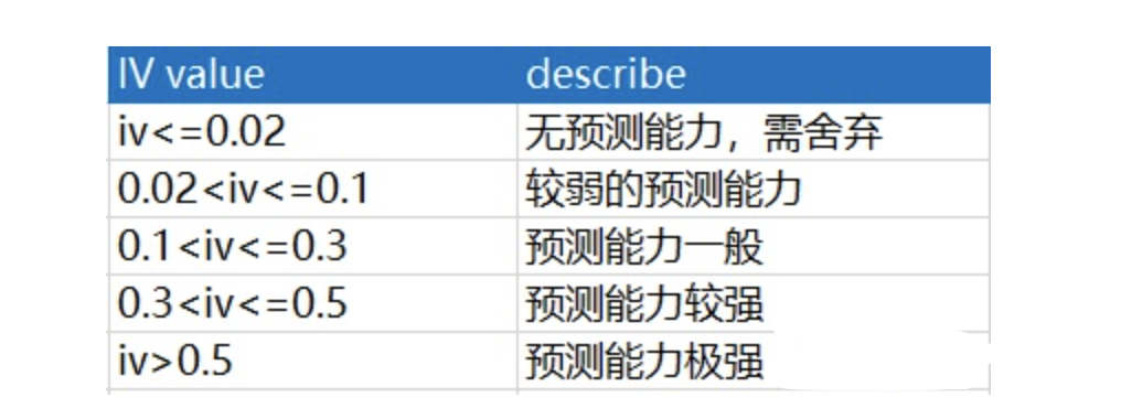
使用Scorecard包中的IV函数计算信息值.

info_value = iv(germancredit, y = "creditability")

info_value

##                                                     variable   info_value
##  1:                      status.of.existing.checking.account 6.660115e-01
##  2:                                        duration.in.month 3.345035e-01
##  3:                                           credit.history 2.932335e-01
##  4:                                             age.in.years 2.596514e-01
##  5:                                savings.account.and.bonds 1.960096e-01
##  6:                                                  purpose 1.691951e-01
##  7:                                                 property 1.126383e-01
##  8:                                 present.employment.since 8.643363e-02
##  9:                                                  housing 8.329343e-02
## 10:                                  other.installment.plans 5.761454e-02
## 11:                                           foreign.worker 4.387741e-02
## 12:                                            credit.amount 3.895727e-02
## 13:                              other.debtors.or.guarantors 3.201932e-02
## 14:      installment.rate.in.percentage.of.disposable.income 2.632209e-02
## 15:                  number.of.existing.credits.at.this.bank 1.326652e-02
## 16:                                  personal.status.and.sex 8.839919e-03
## 17:                                                      job 8.762766e-03
## 18:                                                telephone 6.377605e-03
## 19:                                  present.residence.since 3.588773e-03
## 20: number.of.people.being.liable.to.provide.maintenance.for 4.339223e-05

因此可以筛选一批IV值比较大的变量

dt_f = var_filter(germancredit, y="creditability",iv_limit = 0.1)

## [INFO] filtering variables ...

names(dt_f)

## [1] "status.of.existing.checking.account" "duration.in.month"                  
## [3] "credit.history"                      "purpose"                            
## [5] "savings.account.and.bonds"           "property"                           
## [7] "age.in.years"                        "creditability"

还有很多其他类型的特征选择方法，这里不做过多的介绍了。

粗分类与WOE变换

在构建信用评分模型的过程中，还需要对数据进行WOE变换。证据权重（Weight of Evidence，WOE），可以将逻辑回归模型转变成为标准评分卡格式。

WOE的定义如下：

分子是某一个类别里面坏样本的占比，分母是此类别下好样本的占比，如果括号内的比值小于1，则此类别下坏样本的占比低于好样本的占比，WOE是负数，反之是正数。

需要注意的是，对于连续变量，要计算WOE值，需要先分箱，分箱的方法有很多，等距分箱，等比分箱，另外一种是使用决策树进行分箱：

bins = woebin(germancredit, y="creditability",method = 'tree')

## [INFO] creating woe binning ...

bins$age.in.years

##        variable       bin count count_distr neg pos   posprob        woe
## 1: age.in.years [-Inf,26)   190       0.190 110  80 0.4210526  0.5288441
## 2: age.in.years   [26,28)   101       0.101  74  27 0.2673267 -0.1609304
## 3: age.in.years   [28,35)   257       0.257 172  85 0.3307393  0.1424546
## 4: age.in.years   [35,37)    79       0.079  67  12 0.1518987 -0.8724881
## 5: age.in.years [37, Inf)   373       0.373 277  96 0.2573727 -0.2123715
##         bin_iv  total_iv breaks is_special_values
## 1: 0.057921024 0.1304985     26             FALSE
## 2: 0.002528906 0.1304985     28             FALSE
## 3: 0.005359008 0.1304985     35             FALSE
## 4: 0.048610052 0.1304985     37             FALSE
## 5: 0.016079553 0.1304985    Inf             FALSE

对于age.in.years 的第一个类别，其WOE值为0.5288441，我们来回顾一下是如何计算的：

此类别下，坏样本占总的坏样本的比例：80/(80+27+85+12+96) = 0.2666667
此类别下，好样本占总的好样本的比例：110/(110+74+172+67+277) = 0.1571429
套用公式：log(0.2666667/0.1571429)

WOE变换的优点：

对缺失值不敏感
对极端值不明感
务解释性：我们习惯于线性判断变量的作用，当x越来越大，y就越来越大。但实际x与y之间经常存在着非线性关系，此时可经过WOE变换。

构建模型

构建模型其实很简单，这里就不做过多介绍。

模型评估

混淆矩阵
KS
ROC

PSI稳定性检验

群体稳定性指标(population stability index)公式：

psi = sum(（实际占比-预期占比）* ln(实际占比/预期占比))

举个例子解释下，比如训练一个logistic回归模型，预测时候会有个类概率输出，p。

在你的测试数据集上的输出设定为p1，将它从小到大排序后将数据集10等分（每组样本数一直，此为等宽分组），计算每等分组的最大最小预测的类概率值。

现在你用这个模型去对新的样本进行预测，预测结果叫p2，利用刚才在测试数据集上得到的10等分每等分的上下界。按p2将新样本划分为10分，这个时候不一定是等分了。实际占比就是新样本通过p2落在p1划分出来的每等分界限内的占比，预期占比就是测试数据集上各等分样本的占比。

意义就是如果模型更稳定，那么在新的数据上预测所得类概率应该更建模分布一致，这样落在建模数据集所得的类概率所划分的等分区间上的样本占比应该和建模时一样，否则说明模型变化，一般来自预测变量结构变化。

通常用作模型效果监测。一般认为PSI小于0.1时候模型稳定性很高，0.1-0.2一般，需要进一步研究，大于0.2模型稳定性差，建议修复。

代码实现

scorecard包中的perf_eva函数可以非常方便的进行模型评价,其可以进行更多指标的评估：

data("germancredit")


# var_filter 可以根据制定的标准筛选特征，默认的是筛选IV值大于0.02，缺失率小于0.95，
# identical value rate 小于0.95

dt_f = var_filter(germancredit, y="creditability")

## [INFO] filtering variables ...

# 划分数据集合

dt_list = split_df(dt_f, y="creditability", ratio = 0.6, seed = 30)

## Warning in split_df(dt_f, y = "creditability", ratio = 0.6, seed = 30): The
## ratios is set to c(0.6, 0.4)

#  获取样本的标签
label_list = lapply(dt_list, function(x) x$creditability)


# 进行Woe 分箱,默认的使用方法是树方法

bins = woebin(dt_f, y="creditability") # 这里可以得出分箱，以及WOE变换的详细信息

## [INFO] creating woe binning ...

# 还可以制定划分的方式

breaks_adj = list(
  age.in.years=c(26, 35, 40),
  other.debtors.or.guarantors=c("none", "co-applicant%,%guarantor"))

bins_adj = woebin(dt_f, y="creditability", breaks_list=breaks_adj)

## [INFO] creating woe binning ...

## Warning in check_breaks_list(breaks_list, xs): There are 11 x variables that are
## not specified in breaks_list, and instead are using optimal binning.

# 进行将数据转换成为WOE的值
dt_woe_list = lapply(dt_list, function(x) woebin_ply(x, bins_adj))

## [INFO] converting into woe values ... 
## [INFO] converting into woe values ...

# 建立逻辑回归模型

m1 = glm( creditability ~ ., family = binomial(), data = dt_woe_list$train)

# 逐步回归
m_step = step(m1, direction="both", trace = FALSE)

m2 = eval(m_step$call)




# 进行预测
pred_list = lapply(dt_woe_list, function(x) predict(m2, x, type='response'))

# 模型的评价结果
perf = perf_eva(pred = pred_list$train,label = label_list$train,show_plot = c('ks', 'lift', 'gain', 'roc', 'lz', 'pr', 'f1', 'density'))

## Warning: `guides(<scale> = FALSE)` is deprecated. Please use `guides(<scale> =
## "none")` instead.

## Warning: `guides(<scale> = FALSE)` is deprecated. Please use `guides(<scale> =
## "none")` instead.

## Warning: `guides(<scale> = FALSE)` is deprecated. Please use `guides(<scale> =
## "none")` instead.

## Warning: `guides(<scale> = FALSE)` is deprecated. Please use `guides(<scale> =
## "none")` instead.

perf

## $binomial_metric
## $binomial_metric$dat
##          MSE      RMSE   LogLoss        R2        KS       AUC      Gini
## 1: 0.1493541 0.3864636 0.4562079 0.2751045 0.5517677 0.8232513 0.6465025
## 
## 
## $pic
## TableGrob (3 x 3) "arrange": 8 grobs
##   z     cells    name           grob
## 1 1 (1-1,1-1) arrange gtable[layout]
## 2 2 (1-1,2-2) arrange gtable[layout]
## 3 3 (1-1,3-3) arrange gtable[layout]
## 4 4 (2-2,1-1) arrange gtable[layout]
## 5 5 (2-2,2-2) arrange gtable[layout]
## 6 6 (2-2,3-3) arrange gtable[layout]
## 7 7 (3-3,1-1) arrange gtable[layout]
## 8 8 (3-3,2-2) arrange gtable[layout]

card = scorecard(bins_adj, m2)
score_list = lapply(dt_list, function(x) scorecard_ply(x, card))
perf_psi(score = score_list, label = label_list)

## $pic
## $pic$score

## 
## 
## $psi
##    variable    dataset      psi
## 1:    score train_test 0.048007

评分卡开发

接下来，我们会讲解在模型建立好之后，得到了用户的拒收概率，如何实现一个评分卡。

将估计的违约概率表示为p，则估计的正常概率为1-p，因此：

odds = p / (1 - p)

或者

p = odds / (1 + odds)

评分卡的刻度则是这样表示的:

Score = A - Blog(odds)

其中，A和B是常数，负号使得违约概率越低，得分越高

逻辑回归模型的比率计算公式如下：

也就是说通过逻辑回归模型我们可以得到，p或者odds，其实任何模型都可以得到p，那么我们只要设定好A，B就可以得到具体的评分了，接下来我们介绍如何求得A，B.

计算常数A，B

计算A，B需要假设两个已知的分值代入公式进行计算，通常，需要两个假设：

某个特定比率的预期分值
指定比率翻番的分数（pdo）

假设比率为odds的时候，分值为p1 。然后比率为2*odds的时候，其分值为p1+pdo

那么，代入公式：

p1 = A - B*log(odds)
p1+pdo = A - B*log(2*odds)

解方程得到：

B = pdo/log(2)
A = p1 + B*log(odds)

这样就可以从每一个人的违约概率，得到每一个人的分值。需要注意的是，需要指定几个参数：

某个特定比率的预期分值
指定比率翻番的分数（pdo）

分值分配

我们还需要知道每一个变量的分数是如何影响总的分数的，每一个变量的每一个值的分数计算公式下面给出来：

假设变量x有k个取值，那么，变量x的每一个取值的计算公式为：

- B*(x对应的模型系数)*（x第k个取值的WOE值）

使用R和python时间信用评分模型

scorecard包是在R中提供了一个完整的信用评分模型开发的解决方案。本节会对这一部分内容做一个详细的讲解

首先是现在安装:

install.packages(scorecard)
require(scorecard)

split_df 划分数据集

这个函数是用于划分数据集，使用方法如下:

split_df(dt, y = NULL, ratio = 0.7, seed = 618)

y表示样本的标签，或者说是因变量
ratio 代表的是训练集合与测试集合的比例

data(germancredit)

# Example I
dt_list = split_df(germancredit, y="creditability")
train = dt_list[[1]]
test = dt_list[[2]]


dim(germancredit)

## [1] 1000   21

IV 计算信息值

使用这个函数来计算特征的IV值，用于特征选择作为参考，使用方法如下：

iv(dt, y, x = NULL, positive = "bad|1", order = TRUE)

x表示因变量，默认表示计算所有的自变量的IV
order 表示根据IV进行排序

data(germancredit)

# information values
info_value = iv(germancredit, y = "creditability")
info_value

var_filter 筛选变量

通过设定标准，使用这个函数可以通过特定的标准，信息值，缺失率，筛选特征，使用方法如下:

var_filter(dt, y, x = NULL, iv_limit = 0.02, missing_limit = 0.95,
  identical_limit = 0.95, var_rm = NULL, var_kp = NULL,
  return_rm_reason = FALSE, positive = "bad|1")

1.iv_limit 表示信息值超过多少，才保留此特征，默认是大于0.02 2.missing_limit 表示保留某个缺失率以下的特征，默认是0.95 3.identical_limit 表示，如果某个特征的值一样的比例小于某个比例，则保留，默认是0.95

data(germancredit)

# variable filter
dt_sel = var_filter(germancredit, y = "creditability")

## [INFO] filtering variables ...

names(dt_sel)

##  [1] "status.of.existing.checking.account"                
##  [2] "duration.in.month"                                  
##  [3] "credit.history"                                     
##  [4] "purpose"                                            
##  [5] "credit.amount"                                      
##  [6] "savings.account.and.bonds"                          
##  [7] "present.employment.since"                           
##  [8] "installment.rate.in.percentage.of.disposable.income"
##  [9] "other.debtors.or.guarantors"                        
## [10] "property"                                           
## [11] "age.in.years"                                       
## [12] "other.installment.plans"                            
## [13] "housing"                                            
## [14] "creditability"

woebin 进行WOE变换

使用这个函数进行WOE进行连续变量WOE分箱，使用方法如下：

woebin(dt, y, x = NULL, var_skip = NULL, breaks_list = NULL,
  special_values = NULL, stop_limit = 0.1, count_distr_limit = 0.05,
  bin_num_limit = 8, positive = "bad|1", no_cores = NULL,
  print_step = 0L, method = "tree", save_breaks_list = NULL,
  ignore_const_cols = TRUE, ignore_datetime_cols = TRUE,
  check_cate_num = TRUE, replace_blank_na = TRUE, ...)

1.method 是使用分箱的方法，默认是使用决策树 2.breaks list 可以制定自己的分箱规则 3.stop_limit 如果使用树方法，当信息值增益比小于stop_limit时停止分箱分段; 4.如果使用chimerge方法，当最小卡方大于’qchisq（1-stoplimit，1）’时停止合并。可接受的范围：0-0.5; 默认值为0.1。

bins2_tree = woebin(germancredit, y="creditability", method="tree")

## [INFO] creating woe binning ...

bins2_tree$status.of.existing.checking.account

##                               variable
## 1: status.of.existing.checking.account
## 2: status.of.existing.checking.account
## 3: status.of.existing.checking.account
##                                                       bin count count_distr neg
## 1:                         ... < 0 DM%,%0 <= ... < 200 DM   543       0.543 303
## 2: ... >= 200 DM / salary assignments for at least 1 year    63       0.063  49
## 3:                                    no checking account   394       0.394 348
##    pos   posprob        woe      bin_iv total_iv
## 1: 240 0.4419890  0.6142040 0.225500603 0.639372
## 2:  14 0.2222222 -0.4054651 0.009460853 0.639372
## 3:  46 0.1167513 -1.1762632 0.404410499 0.639372
##                                                    breaks is_special_values
## 1:                         ... < 0 DM%,%0 <= ... < 200 DM             FALSE
## 2: ... >= 200 DM / salary assignments for at least 1 year             FALSE
## 3:                                    no checking account             FALSE

woebin_ply 将原始数据转换成为WOE数据

WOE分箱的具体划分规则指定好了，使用woebin_ply将原始数据转化成为WOE数据，使用方法如下:

woebin_ply(dt, bins, no_cores = NULL, print_step = 0L,
  replace_blank_na = TRUE, ...)

1.dt 是原始数据 2.bins 是woebin 的返回结果

dt_woe = woebin_ply(germancredit, bins=bins2_tree)

## [INFO] converting into woe values ...

head(dt_woe)

##    creditability status.of.existing.checking.account_woe duration.in.month_woe
## 1:          good                                0.614204            -1.3121864
## 2:           bad                                0.614204             1.1349799
## 3:          good                               -1.176263            -0.3466246
## 4:          good                                0.614204             0.5245245
## 5:           bad                                0.614204             0.1086883
## 6:          good                               -1.176263             0.5245245
##    credit.history_woe purpose_woe credit.amount_woe
## 1:        -0.73374058  -0.4100628        0.03366128
## 2:         0.08831862  -0.4100628        0.39053946
## 3:        -0.73374058   0.2799201       -0.25830746
## 4:         0.08831862   0.2799201        0.39053946
## 5:         0.08515781   0.2799201        0.39053946
## 6:         0.08831862   0.2799201        0.39053946
##    savings.account.and.bonds_woe present.employment.since_woe
## 1:                    -0.7621401                  -0.23556607
## 2:                     0.2713578                   0.03210325
## 3:                     0.2713578                  -0.39441527
## 4:                     0.2713578                  -0.39441527
## 5:                     0.2713578                   0.03210325
## 6:                    -0.7621401                   0.03210325
##    installment.rate.in.percentage.of.disposable.income_woe
## 1:                                              0.15730029
## 2:                                             -0.19047277
## 3:                                             -0.19047277
## 4:                                             -0.19047277
## 5:                                             -0.06453852
## 6:                                             -0.19047277
##    personal.status.and.sex_woe other.debtors.or.guarantors_woe
## 1:                  -0.3053816                      0.02797385
## 2:                  -0.3053816                      0.02797385
## 3:                  -0.3053816                      0.02797385
## 4:                  -0.3053816                     -0.58778666
## 5:                  -0.3053816                      0.02797385
## 6:                  -0.3053816                      0.02797385
##    present.residence.since_woe property_woe age.in.years_woe
## 1:                 0.001152738  -0.46103496       -0.2123715
## 2:                 0.070150705  -0.46103496        0.5288441
## 3:                -0.054941118  -0.46103496       -0.2123715
## 4:                 0.001152738   0.02857337       -0.2123715
## 5:                 0.001152738   0.58608236       -0.2123715
## 6:                 0.001152738   0.58608236       -0.8724881
##    other.installment.plans_woe housing_woe
## 1:                  -0.1211786  -0.1941560
## 2:                  -0.1211786  -0.1941560
## 3:                  -0.1211786  -0.1941560
## 4:                  -0.1211786   0.4726044
## 5:                  -0.1211786   0.4726044
## 6:                  -0.1211786   0.4726044
##    number.of.existing.credits.at.this.bank_woe     job_woe
## 1:                                  -0.1347806 -0.02278003
## 2:                                   0.0748775 -0.02278003
## 3:                                   0.0748775 -0.07847162
## 4:                                   0.0748775 -0.02278003
## 5:                                  -0.1347806 -0.02278003
## 6:                                   0.0748775 -0.07847162
##    number.of.people.being.liable.to.provide.maintenance.for_woe telephone_woe
## 1:                                                   0.00281611   -0.09863759
## 2:                                                   0.00281611    0.06469132
## 3:                                                  -0.01540863    0.06469132
## 4:                                                  -0.01540863    0.06469132
## 5:                                                  -0.01540863    0.06469132
## 6:                                                  -0.01540863   -0.09863759
##    foreign.worker_woe
## 1:                  0
## 2:                  0
## 3:                  0
## 4:                  0
## 5:                  0
## 6:                  0

scorecard 构建评分卡

使用scorecard通过模型和woebin的结果构建出评分卡规则，使用方法如下：

scorecard(bins, model, points0 = 600, odds0 = 1/19, pdo = 50,
  basepoints_eq0 = FALSE)

1.bins 是woebin的返回结果 2.model 是构建好的逻辑回归模型 3.odds 比率 4.pdo 增加的分数 5. points0 基础分数

dt_woe$creditability <- as.character(dt_woe$creditability)
dt_woe$creditability[as.character(dt_woe$creditability)=='good']=0
dt_woe$creditability[as.character(dt_woe$creditability)=='bad']=1
dt_woe$creditability <- as.factor(dt_woe$creditability)
l <- glm(creditability~.,data = dt_woe,family = binomial())

score <- scorecard(bins = bins2_tree,model = l)

score$status.of.existing.checking.account

##                               variable
## 1: status.of.existing.checking.account
## 2: status.of.existing.checking.account
## 3: status.of.existing.checking.account
##                                                       bin count count_distr neg
## 1:                         ... < 0 DM%,%0 <= ... < 200 DM   543       0.543 303
## 2: ... >= 200 DM / salary assignments for at least 1 year    63       0.063  49
## 3:                                    no checking account   394       0.394 348
##    pos   posprob        woe      bin_iv total_iv
## 1: 240 0.4419890  0.6142040 0.225500603 0.639372
## 2:  14 0.2222222 -0.4054651 0.009460853 0.639372
## 3:  46 0.1167513 -1.1762632 0.404410499 0.639372
##                                                    breaks is_special_values
## 1:                         ... < 0 DM%,%0 <= ... < 200 DM             FALSE
## 2: ... >= 200 DM / salary assignments for at least 1 year             FALSE
## 3:                                    no checking account             FALSE
##    points
## 1:    -36
## 2:     23
## 3:     68

scorecard_ply

将一个新用户的原始数据获取这个用户的分数，使用方法如下：

scorecard_ply(dt, card, only_total_score = TRUE, print_step = 0L,
  replace_blank_na = TRUE, var_kp = NULL)

dt 训练模型的原始数据集
使用scorecard 建立起来的评分卡规则

resutl <- scorecard_ply(dt = germancredit,card = score)
resutl

##       score
##    1:    NA
##    2:    NA
##    3:    NA
##    4:    NA
##    5:    NA
##   ---      
##  996:    NA
##  997:    NA
##  998:    NA
##  999:    NA
## 1000:    NA

这样就得到了每一个用户的分数

使用python实现

# Traditional Credit Scoring Using Logistic Regression
import scorecardpy as sc

# data prepare ------
# load germancredit data
dat = sc.germancredit()

# filter variable via missing rate, iv, identical value rate
dt_s = sc.var_filter(dat, y="creditability")

# breaking dt into train and test

## [INFO] filtering variables ...
## 
## /Users/milin/.virtualenvs/r-reticulate/lib/python3.8/site-packages/scorecardpy/condition_fun.py:113: UserWarning: The positive value in "creditability" was replaced by 1 and negative value by 0.
##   warnings.warn("The positive value in \"{}\" was replaced by 1 and negative value by 0.".format(y))

train, test = sc.split_df(dt_s, 'creditability').values()

# woe binning ------
bins = sc.woebin(dt_s, y="creditability")
# sc.woebin_plot(bins)

# binning adjustment
# # adjust breaks interactively
# breaks_adj = sc.woebin_adj(dt_s, "creditability", bins) 
# # or specify breaks manually

## [INFO] creating woe binning ...

breaks_adj = {
    'age.in.years': [26, 35, 40],
    'other.debtors.or.guarantors': ["none", "co-applicant%,%guarantor"]
}
bins_adj = sc.woebin(dt_s, y="creditability", breaks_list=breaks_adj)

# converting train and test into woe values

## [INFO] creating woe binning ...

train_woe = sc.woebin_ply(train, bins_adj)

## [INFO] converting into woe values ...

test_woe = sc.woebin_ply(test, bins_adj)

## [INFO] converting into woe values ...

y_train = train_woe.loc[:,'creditability']
X_train = train_woe.loc[:,train_woe.columns != 'creditability']
y_test = test_woe.loc[:,'creditability']
X_test = test_woe.loc[:,train_woe.columns != 'creditability']

# logistic regression ------
from sklearn.linear_model import LogisticRegression
lr = LogisticRegression(penalty='l1', C=0.9, solver='saga', n_jobs=-1)
lr.fit(X_train, y_train)
# lr.coef_
# lr.intercept_

# predicted proability

## LogisticRegression(C=0.9, n_jobs=-1, penalty='l1', solver='saga')

train_pred = lr.predict_proba(X_train)[:,1]
test_pred = lr.predict_proba(X_test)[:,1]

# performance ks & roc ------
train_perf = sc.perf_eva(y_train, train_pred, title = "train")

## /Users/milin/.virtualenvs/r-reticulate/lib/python3.8/site-packages/scorecardpy/perf.py:318: MatplotlibDeprecationWarning: Passing non-integers as three-element position specification is deprecated since 3.3 and will be removed two minor releases later.
##   plt.subplot(subplot_nrows,subplot_ncols,i+1)
## /Users/milin/.virtualenvs/r-reticulate/lib/python3.8/site-packages/scorecardpy/perf.py:318: MatplotlibDeprecationWarning: Passing non-integers as three-element position specification is deprecated since 3.3 and will be removed two minor releases later.
##   plt.subplot(subplot_nrows,subplot_ncols,i+1)

test_perf = sc.perf_eva(y_test, test_pred, title = "test")

# score ------

## /Users/milin/.virtualenvs/r-reticulate/lib/python3.8/site-packages/scorecardpy/perf.py:318: MatplotlibDeprecationWarning: Passing non-integers as three-element position specification is deprecated since 3.3 and will be removed two minor releases later.
##   plt.subplot(subplot_nrows,subplot_ncols,i+1)
## /Users/milin/.virtualenvs/r-reticulate/lib/python3.8/site-packages/scorecardpy/perf.py:318: MatplotlibDeprecationWarning: Passing non-integers as three-element position specification is deprecated since 3.3 and will be removed two minor releases later.
##   plt.subplot(subplot_nrows,subplot_ncols,i+1)

card = sc.scorecard(bins_adj, lr, X_train.columns)
# credit score
train_score = sc.scorecard_ply(train, card, print_step=0)

## /Users/milin/.virtualenvs/r-reticulate/lib/python3.8/site-packages/pandas/core/indexing.py:1951: SettingWithCopyWarning: 
## A value is trying to be set on a copy of a slice from a DataFrame.
## Try using .loc[row_indexer,col_indexer] = value instead
## 
## See the caveats in the documentation: https://pandas.pydata.org/pandas-docs/stable/user_guide/indexing.html#returning-a-view-versus-a-copy
##   self.obj[selected_item_labels] = value
## /Users/milin/.virtualenvs/r-reticulate/lib/python3.8/site-packages/pandas/core/indexing.py:1667: SettingWithCopyWarning: 
## A value is trying to be set on a copy of a slice from a DataFrame.
## Try using .loc[row_indexer,col_indexer] = value instead
## 
## See the caveats in the documentation: https://pandas.pydata.org/pandas-docs/stable/user_guide/indexing.html#returning-a-view-versus-a-copy
##   self.obj[key] = value

test_score = sc.scorecard_ply(test, card, print_step=0)

# psi
sc.perf_psi(
  score = {'train':train_score, 'test':test_score},
  label = {'train':y_train, 'test':y_test}
)

## {'psi':   variable       PSI
## 0    score  0.008984, 'pic': {'score': <Figure size 700x500 with 0 Axes>}}

信用评分模型开发

Liam

11/6/2021

敏捷数据科学

目录

评分卡开发流程

评分卡

标准评分卡

正常与违约

标准评分卡的格式

信用评分卡的优点

评分卡开发流程

数据准备

探索性分析

特征选择

模型开发

模型验证

分卡开发

模型的上线与监控

数据获取与数据整合

信用评分卡的数据来源

完整性检验

探索性分析

变量的分布情况

列联表分析

极端值的识别

特征选择

粗分类与WOE变换

构建模型

模型评估

PSI稳定性检验

代码实现

评分卡开发

计算常数A，B

分值分配

使用R和python时间信用评分模型

split_df 划分数据集

IV 计算信息值

var_filter 筛选变量

woebin 进行WOE变换

woebin_ply 将原始数据转换成为WOE数据

scorecard 构建评分卡

scorecard_ply

使用python实现