Given:
\[\sigma = 1.25 \\ n = 10 \\ \overline{x} = 40.5 \\ \alpha = 0.06\]
From the question, our hypotheses should be:
\[H_0 = \mu = 40 \\ H_a = \mu > 40\]
The first thing to do is to get the z-value at 40.
\[z = \frac{x - \mu}{\frac{\sigma}{\sqrt{n}}} \\ z = \frac{40.5 - 40}{\frac{1.25}{\sqrt{10}}} \\ z = \frac{0.5}{\frac{1.25}{\sqrt{10}}} \\ z = 1.265 \\ z = 1.26\]
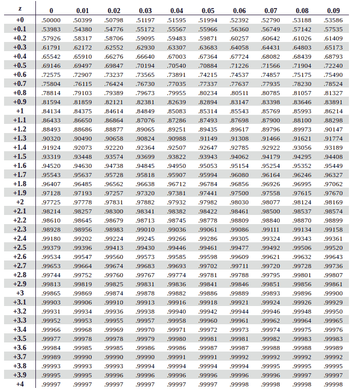
To check whether the claim is true, we will compare the P-value to the given significance value. The Z-score can be obtained from a Z Table.
\[ \mathrm{P_v} = (Z > 1.26) \\ \mathrm{P_v} = 1 - (Z < 1.26) \\ \mathrm{P_v} = 1 - (0.89617) \\ \mathrm{P_v} = 0.10383\]
Since the P-value is greater than the significance level, \[ 0.10383 > 0.05 \] Therefore there is enough evidence to reject the Null hypothesis \(H_0\).
Stating the claim that battery life exceeds 40 hours is true.
Since the P-value is the one used for Question A, the solution will be the same.
\[ \mathrm{P_v} = (Z > 1.26) \\ \mathrm{P_v} = 1 - (Z < 1.26) \\ \mathrm{P_v} = 1 - (0.89617) \\ \mathrm{P_v} = 0.10383\]
The P-value is 0.10383.
The formula to get the probability of a \(\beta\)-error in a one-sided or one-tailed test is:
\[\beta = \mathrm{P}(Z < Z_\alpha - \frac{(x-\mu)\sqrt{n}}{\sigma})\] In this formula, we will substitute \(x = 42\) as it is given as the true mean life.
\[ \beta = \mathrm{P}(Z < 1.645 - \frac{(42-40)\sqrt{10}}{1.25})\] 1.645 is the z-value of when \(\alpha\) = 0.05.
qnorm(0.05, lower.tail=FALSE)## [1] 1.644854\[\beta = \mathrm{P}(Z < 1.645 - \frac{(2)\sqrt{10}}{1.25}) \\ \beta = \mathrm{P}(Z < 1.645 - 5.059) \\ \beta = \mathrm{P}(Z < -3.414) \\ \beta = 0.00032\]
To conclude, the Beta (\(\beta\)) or Type-II error when the true mean is 42 is 0.00032.
In this problem, the true mean is now 44. Here is the formula given:
\[n = \frac{(Z_\alpha-Z_\beta)(\sigma^{2})}{\delta^{2}}\] As we do not want \(\beta\) to exceed 0.10,
\[Z_1 - Z_{0.1} = Z_{0.9} = 1.28\]
qnorm(0.9)## [1] 1.281552Therefore, \(Z_\beta = 1.28\).
\[n = \frac{(1.65+1.28)^{2}(1.25^{2})}{(44-40)^{2}} \\ n = \frac{(2.93)^{2}(1.25^{2})}{(4)^{2}} \\ n = \frac{(8.5849)(1.5625)}{16} \\ n = \frac{13.4139}{16} \\ n = 0.838\]
\(0.838 ≈ 1\)
To ensure that the \(\beta\) value does not exceed 0.1 if the true mean is 44 hours, the sample mean should be 1.
For a one-sided test, we can use the equation (see figure below) to identify the right side of the interval.
\[\overline{x} + Z_\alpha(\frac{\sigma}{\sqrt{n}})\] Substituting the values:
\[ 40.5 +1.65(\frac{1.25}{\sqrt{10}}) \\ 40.5 + 0.6522 \\ =41.15\]
Knowing that this is a one-sided test leaves us with an interval of confidence of
\[(-\infty,41.15)\] And since the value 40 is inside the interval, like in Question A, there is not enough evidence to reject the null hypothesis.
Given:
Brand A GasolineApplying the Seven-Step hypothesis-testing process:
Since we are testing whether Gasoline B has a better mileage than Gasoline A, therefore the parameter of interest of this problem would be the two brand’s mean mileage which we will represent here as \(\mu_a\) and \(\mu_b\).
\[ H_0 = \mu_a = \mu_b \]
\[ H_a = \mu_b > \mu_a \]
\[ t = \frac{{\overline{x}_a - \overline{x}_b-\Delta_0}}{\sqrt {\frac{(\sigma_a)^2}{n_a} + \frac{(\sigma_b)^2}{n_b}}}\]
Other formulas:
Getting the Degree of Freedom
\[D_f = \frac{((\frac{\sigma_a^2}{n_a})+(\frac{\sigma_b^2}{n_b}))^2}{\frac{(\frac{\sigma_a^2}{n_a})^2}{n_a-1}+\frac{(\frac{\sigma_b^2}{n_b})^2}{n_b-1}}\]
We will reject \(H_0\) if the P-value is less than the significance level which is 0.05
\[ P_v < \alpha \] \[ P_v < 0.05 \]
With \(t\) as the t-score, we will reject \(H_0\) if \(t\) is greater than the positive t-critical value or less than the negative t-value.
\[ t > t-value_+ \\ t < t-value_-\]
\[ t = \frac{{\overline{x}_a - \overline{x}_b}}{\sqrt {\frac{(\sigma_a)^2}{n_a} + \frac{(\sigma_b)^2}{n_b}}}\]
Noting that the sample of both brands is 16, therefore both \(n_a\) and \(n_b\) are equal to 16.
\[t = \frac{{19.6 - 20.2}}{\sqrt {\frac{0.4^2}{16} + \frac{0.6^2}{16}}} \\ t = \frac{{-0.6}}{\sqrt {{0.01} + {0.0225}}} \\ t = \frac{{-0.6}}{0.1803} \\ t = \frac{{-0.6}}{0.1803} \\ t = -3.328 \\ = -3.33\]
Getting the Degree of Freedom
\[D_f = \frac{((\frac{\sigma_a^2}{n_a})+(\frac{\sigma_b^2}{n_b}))^2}{\frac{(\frac{\sigma_a^2}{n_a})^2}{n_a-1}+\frac{(\frac{\sigma_b^2}{n_b})^2}{n_b-1}}\] \[D_f = \frac{((\frac{0.4^2}{16})+(\frac{0.6^2}{16}))^2}{\frac{(\frac{0.4^2}{16})^2}{16-1}+\frac{(\frac{0.6^2}{16})^2}{16-1}}\] \[D_f = \frac{((\frac{0.16}{16})+(\frac{0.36}{16}))^2}{\frac{(\frac{0.16}{16})^2}{15}+\frac{(\frac{0.36}{16})^2}{15}}\] \[D_f = \frac{(0.01+0.0225)^2}{\frac{(0.01)^2}{15}+\frac{(0.0225)^2}{15}}\] \[D_f = \frac{(0.0325)^2}{\frac{0.0001}{15}+\frac{0.00050625}{15}}\] \[D_f = \frac{0.00105625}{\frac{0.00060625}{15}}\] \[D_f = 26.134 \\ D_f ≈ 26\]
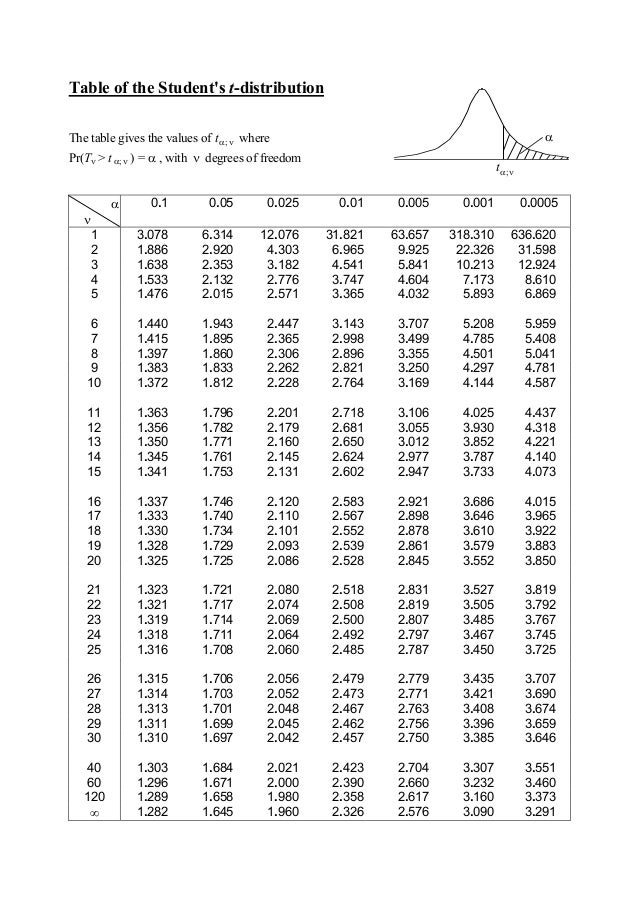
T-Values
After getting the significance level (0.05) and the the degree of freedom (26), we can now obtain the T-Value from a sample table T-critical Values.
\[t-value = 1.706\]
After getting the t-score and degree of freedom, we calculate the P-value:
\[\mathrm{P} = \phi(-3.33) \\ \mathrm{P} = 0.001303\]
pt(-3.33, 26, lower.tail = TRUE)## [1] 0.001302654We will reject \(H_0\) if the P-value is less than the Significance level which is 0.05
\[ P_v < \alpha \] \[ P_v < 0.05 \] \[ 0.0013 < 0.05\]
Therefore the condition to reject the null hypothesis \(H_0\) is obtained.
With \(t\) as the t-score, we will reject \(H_0\) if \(t\) is greater than the positive t-critical value or less than the negative t-critical value.
\[ t = -3.33 \\ t-value = ± 2.056\]
Since the t-score is negative, we’ll compare it with the negative t-critical value.
\[ t < t-value_- \\ -3.33 < -2.056\]
Therefore the condition to reject the null hypothesis \(H_0\) is obtained.
Since the requirements to reject the null hypothesis (\(H_0\)) has been achieved in both tests, the null hypothesis shall be acclaimed as false.
Stating that the mileage of Gasoline B is significantly better than that of Gasoline A.
Montgomery, D. C., & Runger, G. C. (2019). 10 Statistical Inference for Two Samples. In Applied Statistics and Probability for Engineers (7th ed., pp. 262–279). essay, Wiley.
Book Link.