• Take some time to set up your screen
  • RStudio, Zoom window, Zoom chat, maybe a web browser
• Leave your camera on if you are comfortable
• Feel free to ask questions by:
  • Unmuting, raising hand, putting question in chat…
• Don’t hesitate to ask questions!

1. Why is text different?
2. What is tidy text?
3. Tokenizing and counting words
4. Sentiment analysis
5. Term frequency * inverse document frequency
6. n-grams and beyond

NOTE: We’ll have a break about halfway through!

Text Mining with R: A Tidy Approach

• why is text data called “unstructured”?
• what issues are common with text data?
• where can you get text data for your work?

• remember tidy data principles?
  1. Each variable has its own column
  2. Each observation has its own row
  3. Each value must have its own cell
• for text data, this means a table with one token per row
• not all text mining work can use tidy format, some other formats are:
  1. Strings – i.e., character vectors (often the way text is imported)
  2. Corpus – strings annotated with additional metadata
  3. Document-term matrix – a matrix describing a collection of documents with one document per row, one column for each term

text_df %>%
  unnest_tokens(word, text)

• text is split into tokens (default is words)
• other columns are retained
• punctuation is stripped
• by default, unnest_tokens() converts the tokens to lowercase, which makes them easier to compare or combine with other datasets (Use the to_lower = FALSE argument to turn off this behavior)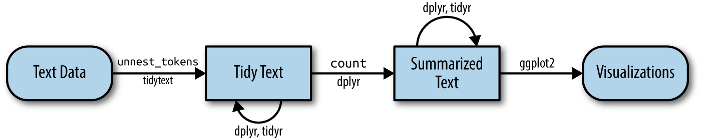

Use what we’ve just learned to a create a bar chart of the 15 least used words that are used over 100 times in the Jane Austen corpus.

Hint: the tail() function might be quite useful here.

When you’re done, please give a :thumbs-up: or a :green-check: in the Zoom reactions.

Modify the code we used before for the most used words in the Jane Austen corpus so that we can see a separate graph of the most used words in each of the books in the corpus.

Hint: the facet_grid() function is important here.

When you’re done, please give a :thumbs-up: or a :green-check: in the Zoom reactions.

install.packages('gutenbergr')
library(gutenbergr)
gutenberg_metadata
View(gutenberg_metadata)

• check out the package’s documentation at rOpenSci, where it is one of rOpenSci’s packages for data access.
• we’ll be using the gutenberg_download() function to download work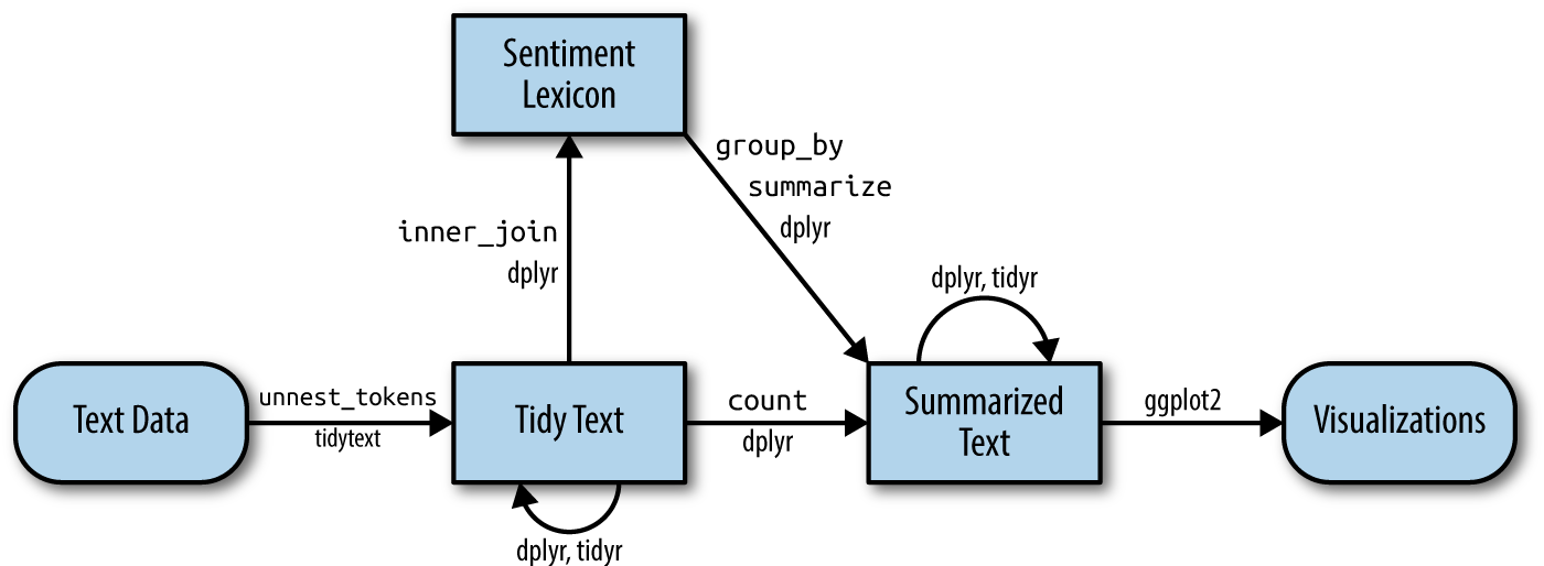s

• AFINN from Finn Årup Nielsen
• bing from Bing Liu and collaborators
• nrc from Saif Mohammad and Peter Turney

NOTE: These lexicons are available under different licenses, so be sure that the license for the lexicon you want to use is appropriate for your project. You may be asked to agree to a license before downloading data.

library(tidytext)
get_sentiments("afinn")

Use the get_sentiments() function to download each of the 3 datasets (AFINN, bing, and nrc). Make sure to read each license before you accept it.

When you’re done, please give a :thumbs-up: or a :green-check: in the Zoom reactions.

“How were these sentiment lexicons put together and validated? They were constructed via either crowdsourcing (using, for example, Amazon Mechanical Turk) or by the labor of one of the authors, and were validated using some combination of crowdsourcing again, restaurant or movie reviews, or Twitter data. Given this information, we may hesitate to apply these sentiment lexicons to styles of text dramatically different from what they were validated on, such as narrative fiction from 200 years ago. While it is true that using these sentiment lexicons with, for example, Jane Austen’s novels may give us less accurate results than with tweets sent by a contemporary writer, we still can measure the sentiment content for words that are shared across the lexicon and the text.”

• inner_join(): return all rows from x where there are matching values in y, and all columns from x and y. If there are multiple matches between x and y, all combination of the matches are returned.
• anti_join(): return all rows from x where there are not matching values in y, keeping just columns from x.

Other info on these and other types of joins can be found on the documentation page.

The %/% operator does integer division (x %/% y is equivalent to floor(x/y)) so the index keeps track of which 80-line section of text we are counting up negative and positive sentiments in.

Write some code that will add the word “miss” to our stop_words tibble. Call the lexicon “custom.”

HINT: the bind_rows() function will be helpful here.

When you’re done, please give a :thumbs-up: or a :green-check: in the Zoom reactions.

\[idf(\text{term}) = \ln{\left(\frac{n_{\text{documents}}}{n_{\text{documents containing term}}}\right)}\]

NOTE: the statistic tf-idf is a rule-of-thumb quantity; while it is very useful (and widely used) in text mining, its theoretical foundations are regularly questioned by information experts.

The bind_tf_idf() function in the tidytext package takes a tidy text dataset as input with one row per token (term), per document. One column (word for us) contains the terms/tokens, one column contains the documents (book in our case), and the last necessary column contains the counts, how many times each document contains each term (n in our example).

We can add two arguments (token = "ngrams" and n = n) to our unnest_tokens() function in order to capture n-grams (instead of single words, or unigrams).

austen_bigrams <- austen_books() %>%
  unnest_tokens(bigram, text, token = "ngrams", n = 2)

To sign up for more sessions: go/summer-data-workshops/

Assessment survey: go/summer-data-assessment/

Ryan’s contact info: go/ryan/