Using ADHD / MD Questionnaires To Predict Suicide

GOAL

For this assignment, we will be working with a very interesting mental health dataset from a real-life research project. All identifying information, of course, has been removed. The attached spreadsheet has the data (the tab name “Data”). The data dictionary is given in the second tab. You can get as creative as you want. The assignment is designed to really get you to think about how you could use different methods.

Please use a clustering method to find clusters of patients here. Whether you choose to use k-means clustering or hierarchical clustering is up to you as long as you reason through your work. Can you come up with creative names for the profiles you found? (
Let’s explore using Principal Component Analysis on this dataset. You will note that there are different types of questions in the dataset: column: E-W: ADHD self-report; column X – AM: mood disorders questionnaire, column AN-AS: Individual Substance Misuse; etc. Please reason through your work as you decide on which sets of variables you want to use to conduct Principal Component Analysis.
Assume you are modeling whether a patient attempted suicide (column AX). Please use support vector machine to model this. You might want to consider reducing the number of variables or somehow use extracted information from the variables. This can be a really fun modeling task!

HW4 for Machine Learning 622 This is Version6

SETUP

library(skimr)
library(tidymodels)

## -- Attaching packages -------------------------------------- tidymodels 0.1.3 --

## v broom        0.7.6      v recipes      0.1.16
## v dials        0.0.9      v rsample      0.1.0 
## v dplyr        1.0.6      v tibble       3.1.1 
## v ggplot2      3.3.3      v tidyr        1.1.3 
## v infer        0.5.4      v tune         0.1.5 
## v modeldata    0.1.0      v workflows    0.2.2 
## v parsnip      0.1.5      v workflowsets 0.0.2 
## v purrr        0.3.4      v yardstick    0.0.8

## -- Conflicts ----------------------------------------- tidymodels_conflicts() --
## x purrr::discard() masks scales::discard()
## x dplyr::filter()  masks stats::filter()
## x dplyr::lag()     masks stats::lag()
## x recipes::step()  masks stats::step()
## * Use tidymodels_prefer() to resolve common conflicts.

library(visdat)  ## missing visual

library(dplyr)
library(tidyr)
library(ggplot2)
library(tidyverse)

library(caret) # For featureplot, classification report
library(corrplot) # For correlation matrix
library(AppliedPredictiveModeling)
library(mice) # For data imputation
library(VIM) # For missing data visualization
library(gridExtra) # For grid plots
library(pROC) # For AUC calculations
library(ROCR) # For ROC and AUC plots
library(dendextend)
library(factoextra)

library(inspectdf)
library(corrplot)
library(stats)
library(kableExtra)

## 
## Attaching package: 'kableExtra'

## The following object is masked from 'package:dplyr':
## 
##     group_rows

library(kernlab)        # SVM methodology

## 
## Attaching package: 'kernlab'

## The following object is masked from 'package:purrr':
## 
##     cross

## The following object is masked from 'package:ggplot2':
## 
##     alpha

## The following object is masked from 'package:scales':
## 
##     alpha

library(e1071)          # SVM methodology

## 
## Attaching package: 'e1071'

## The following object is masked from 'package:tune':
## 
##     tune

## The following object is masked from 'package:rsample':
## 
##     permutations

library(data.table)

library(CGPfunctions)

## Registered S3 methods overwritten by 'lme4':
##   method                          from
##   cooks.distance.influence.merMod car 
##   influence.merMod                car 
##   dfbeta.influence.merMod         car 
##   dfbetas.influence.merMod        car

DATASET

ADHD/MD QUESTIONNAIRE

ADHD is a neurological disorder that can present itself in adolescence and adulthood. Some individuals can outgrow ADHD but around 30% will continue to have ADHD throughout their adulthood.

The Adult ADHD Self-Report Scale Symptom Checklist is a self-reported questionnaire used to assist in the diagnosis of adult ADHD.

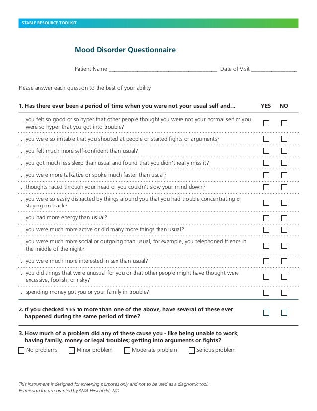
The Mood Disorder Questionnaire is a self-report questionnaire designed to help detect bipolar disorder. It focuses on symptoms of hypomania and mania, which are the mood states that separate bipolar disorders from other types of depression and mood disorder. It has 5 main questions, and the first question has 13 parts, for a total of 17 questions.

Details of the items an answers for the questionnaires are included in link below

https://counsellingresource.com/quizzes/adhd-testing/adhd-asrs/

https://www.apaservices.org/practice/reimbursement/health-registry/self-reporting-sympton-scale.pdf

https://www.healthyplace.com/depression/bipolar/mood-disorders-questionnaire#:~:text=The%20Mood%20Disorder%20Questionnaire%20%28MDQ%29%20was%20developed%20by,-%20it%20is%20not%20considered%20a%20diagnostic%20tool.

https://image.slidesharecdn.com/mdq-160919231357/95/mood-disorder-questionnaire-2-638.jpg?cb=1474326860

DATA DICTIONARY

Initial Respondents initial:
Age Age: 0 … 69
Sex Sex: Male-1, Female-2
Race Race: White-1, African American-2, Hispanic-3, Asian-4, Native American-5, Other or missing data -6
ADHD Q(n) ADHD self-report scale: Never-0, rarely-1, sometimes-2, often-3, very often-4
ADHD Total ADHD self-report Total: Sum of ADHD question scores
MD Q(n) Mood disorder questions: No-0, yes-1; question 3: no problem-0, minor-1, moderate-2, serious-3
MD TOTAL MD self-report Total: Sum of MD question scores
Alcohol Individual substances misuse: no use-0, use-1, abuse-2, dependence-3
THC Individual substances misuse: no use-0, use-1, abuse-2, dependence-3
Cocaine Individual substances misuse: no use-0, use-1, abuse-2, dependence-3
Stimulants Individual substances misuse: no use-0, use-1, abuse-2, dependence-3
Sedative-hypnotics Individual substances misuse: no use-0, use-1, abuse-2, dependence-3
Opioids Individual substances misuse: no use-0, use-1, abuse-2, dependence-3
Court order Court Order: No-0, Yes-1
Education Education: 1-12 grade, 13+ college
Hx of Violence History of Violence: No-0, Yes-1
Disorderly Conduct Disorderly Conduct: No-0, Yes-1
Suicide Suicide attempt: No-0, Yes-1
Abuse Abuse Hx: No-0, Physical (P)-1, Sexual (S)-2, Emotional (E)-3, P&S-4, P&E-5, S&E-6, P&S&E-7
Non-subst Dx Non-substance-related Dx: 0 – none; 1 – one; 2 – More than one
Subst Dx Substance-related Dx: 0 – none; 1 – one Substance-related; 2 – two; 3 – three or more
Psych meds. Psychiatric Meds: 0 – none; 1 – one psychotropic med; 2 – more than one psychotropic med

DATA EXPLORATION

adhd_hw4_notReduced <- read.csv ('adhd_data.csv', header = TRUE) #175*54

head(adhd_hw4_notReduced,5)

tail(adhd_hw4_notReduced,6)

adhd_hw4_notReduced[adhd_hw4_notReduced==''] <- NA 

nrow(is.na(adhd_hw4_notReduced))

## [1] 175

head(adhd_hw4_notReduced,3)

 skim(adhd_hw4_notReduced)

Data summary

Name	adhd_hw4_notReduced
Number of rows	175
Number of columns	54
_______________________
Column type frequency:
factor	1
numeric	53
________________________
Group variables	None

Variable type: factor

skim_variable	n_missing	complete_rate	ordered	n_unique	top_counts
Initial	0	1	FALSE	109	DB: 5, CM: 4, DJ: 4, JM: 4

Variable type: numeric

skim_variable	n_missing	complete_rate	mean	sd	p0	p25	p50	p75	p100	hist
Age	0	1.00	39.47	11.17	18	29.5	42	48.0	69	<U+2586><U+2585><U+2587><U+2585><U+2581>
Sex	0	1.00	1.43	0.50	1	1.0	1	2.0	2	<U+2587><U+2581><U+2581><U+2581><U+2586>
Race	0	1.00	1.64	0.69	1	1.0	2	2.0	6	<U+2587><U+2581><U+2581><U+2581><U+2581>
ADHD.Q1	0	1.00	1.70	1.29	0	1.0	2	3.0	4	<U+2587><U+2587><U+2587><U+2586><U+2583>
ADHD.Q2	0	1.00	1.91	1.25	0	1.0	2	3.0	4	<U+2585><U+2587><U+2587><U+2586><U+2585>
ADHD.Q3	0	1.00	1.91	1.27	0	1.0	2	3.0	4	<U+2585><U+2587><U+2587><U+2586><U+2585>
ADHD.Q4	0	1.00	2.10	1.34	0	1.0	2	3.0	4	<U+2585><U+2585><U+2587><U+2585><U+2586>
ADHD.Q5	0	1.00	2.26	1.44	0	1.0	3	3.0	5	<U+2587><U+2585><U+2587><U+2586><U+2581>
ADHD.Q6	0	1.00	1.91	1.31	0	1.0	2	3.0	4	<U+2586><U+2585><U+2587><U+2587><U+2583>
ADHD.Q7	0	1.00	1.83	1.19	0	1.0	2	3.0	4	<U+2583><U+2587><U+2587><U+2583><U+2583>
ADHD.Q8	0	1.00	2.14	1.29	0	1.0	2	3.0	4	<U+2583><U+2587><U+2587><U+2587><U+2586>
ADHD.Q9	0	1.00	1.91	1.32	0	1.0	2	3.0	4	<U+2586><U+2587><U+2587><U+2587><U+2585>
ADHD.Q10	0	1.00	2.12	1.23	0	1.0	2	3.0	4	<U+2582><U+2587><U+2587><U+2586><U+2585>
ADHD.Q11	0	1.00	2.27	1.24	0	1.0	2	3.0	4	<U+2582><U+2586><U+2587><U+2587><U+2586>
ADHD.Q12	0	1.00	1.29	1.21	0	0.0	1	2.0	4	<U+2587><U+2587><U+2586><U+2582><U+2582>
ADHD.Q13	0	1.00	2.37	1.23	0	1.5	2	3.0	4	<U+2582><U+2585><U+2587><U+2587><U+2586>
ADHD.Q14	0	1.00	2.25	1.35	0	1.0	2	3.0	4	<U+2585><U+2585><U+2587><U+2587><U+2586>
ADHD.Q15	0	1.00	1.63	1.39	0	0.0	1	3.0	4	<U+2587><U+2586><U+2586><U+2585><U+2583>
ADHD.Q16	0	1.00	1.70	1.38	0	1.0	1	3.0	4	<U+2586><U+2587><U+2586><U+2583><U+2585>
ADHD.Q17	0	1.00	1.53	1.29	0	0.0	1	2.0	4	<U+2587><U+2587><U+2587><U+2583><U+2583>
ADHD.Q18	0	1.00	1.47	1.30	0	0.0	1	2.0	4	<U+2587><U+2587><U+2586><U+2583><U+2583>
ADHD.Total	0	1.00	34.32	16.70	0	21.0	33	47.5	72	<U+2583><U+2586><U+2587><U+2586><U+2582>
MD.Q1a	0	1.00	0.55	0.50	0	0.0	1	1.0	1	<U+2586><U+2581><U+2581><U+2581><U+2587>
MD.Q1b	0	1.00	0.57	0.50	0	0.0	1	1.0	1	<U+2586><U+2581><U+2581><U+2581><U+2587>
MD.Q1c	0	1.00	0.54	0.50	0	0.0	1	1.0	1	<U+2587><U+2581><U+2581><U+2581><U+2587>
MD.Q1d	0	1.00	0.58	0.49	0	0.0	1	1.0	1	<U+2586><U+2581><U+2581><U+2581><U+2587>
MD.Q1e	0	1.00	0.55	0.50	0	0.0	1	1.0	1	<U+2586><U+2581><U+2581><U+2581><U+2587>
MD.Q1f	0	1.00	0.70	0.46	0	0.0	1	1.0	1	<U+2583><U+2581><U+2581><U+2581><U+2587>
MD.Q1g	0	1.00	0.72	0.45	0	0.0	1	1.0	1	<U+2583><U+2581><U+2581><U+2581><U+2587>
MD.Q1h	0	1.00	0.56	0.50	0	0.0	1	1.0	1	<U+2586><U+2581><U+2581><U+2581><U+2587>
MD.Q1i	0	1.00	0.59	0.49	0	0.0	1	1.0	1	<U+2586><U+2581><U+2581><U+2581><U+2587>
MD.Q1j	0	1.00	0.39	0.49	0	0.0	0	1.0	1	<U+2587><U+2581><U+2581><U+2581><U+2585>
MD.Q1k	0	1.00	0.49	0.50	0	0.0	0	1.0	1	<U+2587><U+2581><U+2581><U+2581><U+2587>
MD.Q1L	0	1.00	0.58	0.49	0	0.0	1	1.0	1	<U+2586><U+2581><U+2581><U+2581><U+2587>
MD.Q1m	0	1.00	0.49	0.50	0	0.0	0	1.0	1	<U+2587><U+2581><U+2581><U+2581><U+2587>
MD.Q2	0	1.00	0.72	0.45	0	0.0	1	1.0	1	<U+2583><U+2581><U+2581><U+2581><U+2587>
MD.Q3	0	1.00	2.01	1.07	0	1.0	2	3.0	3	<U+2582><U+2582><U+2581><U+2585><U+2587>
MD.TOTAL	0	1.00	10.02	4.81	0	6.5	11	14.0	17	<U+2583><U+2583><U+2586><U+2587><U+2587>
Alcohol	4	0.98	1.35	1.39	0	0.0	1	3.0	3	<U+2587><U+2582><U+2581><U+2581><U+2586>
THC	4	0.98	0.81	1.27	0	0.0	0	1.5	3	<U+2587><U+2581><U+2581><U+2581><U+2583>
Cocaine	4	0.98	1.09	1.39	0	0.0	0	3.0	3	<U+2587><U+2581><U+2581><U+2581><U+2585>
Stimulants	4	0.98	0.12	0.53	0	0.0	0	0.0	3	<U+2587><U+2581><U+2581><U+2581><U+2581>
Sedative.hypnotics	4	0.98	0.12	0.54	0	0.0	0	0.0	3	<U+2587><U+2581><U+2581><U+2581><U+2581>
Opioids	4	0.98	0.39	0.99	0	0.0	0	0.0	3	<U+2587><U+2581><U+2581><U+2581><U+2581>
Court.order	5	0.97	0.09	0.28	0	0.0	0	0.0	1	<U+2587><U+2581><U+2581><U+2581><U+2581>
Education	9	0.95	11.90	2.17	6	11.0	12	13.0	19	<U+2581><U+2585><U+2587><U+2582><U+2581>
Hx.of.Violence	11	0.94	0.24	0.43	0	0.0	0	0.0	1	<U+2587><U+2581><U+2581><U+2581><U+2582>
Disorderly.Conduct	11	0.94	0.73	0.45	0	0.0	1	1.0	1	<U+2583><U+2581><U+2581><U+2581><U+2587>
Suicide	13	0.93	0.30	0.46	0	0.0	0	1.0	1	<U+2587><U+2581><U+2581><U+2581><U+2583>
Abuse	14	0.92	1.33	2.12	0	0.0	0	2.0	7	<U+2587><U+2582><U+2581><U+2581><U+2581>
Non.subst.Dx	22	0.87	0.44	0.68	0	0.0	0	1.0	2	<U+2587><U+2581><U+2583><U+2581><U+2581>
Subst.Dx	23	0.87	1.14	0.93	0	0.0	1	2.0	3	<U+2586><U+2587><U+2581><U+2585><U+2582>
Psych.meds.	118	0.33	0.96	0.80	0	0.0	1	2.0	2	<U+2587><U+2581><U+2587><U+2581><U+2586>

# Selecting only variables not containing Qs
adhd_hw4 <- adhd_hw4_notReduced  %>% select(c(Age, Sex, Race, ADHD.Total, MD.TOTAL, Alcohol:Psych.meds.))
### 175 * 20VR
## Using Reduced ones

adhd_hw4_notReduced.new = apply(adhd_hw4_notReduced, 2, function(x) as.numeric(as.character(x))) %>% 
   data.frame()

## Warning in FUN(newX[, i], ...): NAs introduced by coercion

##NA introduced by coersion

adhd_hw4_notReduced.long<- stack(adhd_hw4_notReduced.new)

head(adhd_hw4_notReduced.long,3)

# https://rpubs.com/ghh2001/699273
ggplot(data = adhd_hw4_notReduced.long, 
       aes(x=as.factor(values),
           fill=as.factor(values) )) +
            geom_bar(stat='count', width=1) +   
              facet_wrap(~ind)

nearZeroVar(adhd_hw4_notReduced, names=TRUE, saveMetrics = T)

MISSING DATA INVESTIGATION

library(visdat)
visdat::vis_miss(adhd_hw4)

mice_plot <- aggr(adhd_hw4_notReduced, col=c('#F8766D','#00BFC4'), numbers=TRUE, sortVars=TRUE, labels=names(adhd_hw4), cex.axis=.7, gap=3, ylab=c("Missing data","Pattern"))

## 
##  Variables sorted by number of missings: 
##            Variable      Count
##      Hx.of.Violence 0.67428571
##           Education 0.13142857
##         Court.order 0.12571429
##             Opioids 0.08000000
##  Sedative.hypnotics 0.07428571
##             Cocaine 0.06285714
##          Stimulants 0.06285714
##                 THC 0.05142857
##             Alcohol 0.02857143
##         Psych.meds. 0.02285714
##                 Age 0.02285714
##                 Sex 0.02285714
##                Race 0.02285714
##          ADHD.Total 0.02285714
##            MD.TOTAL 0.02285714
##                 Age 0.00000000
##                 Sex 0.00000000
##                Race 0.00000000
##          ADHD.Total 0.00000000
##            MD.TOTAL 0.00000000
##             Alcohol 0.00000000
##                 THC 0.00000000
##             Cocaine 0.00000000
##          Stimulants 0.00000000
##  Sedative.hypnotics 0.00000000
##             Opioids 0.00000000
##         Court.order 0.00000000
##           Education 0.00000000
##      Hx.of.Violence 0.00000000
##  Disorderly.Conduct 0.00000000
##             Suicide 0.00000000
##               Abuse 0.00000000
##        Non.subst.Dx 0.00000000
##            Subst.Dx 0.00000000
##         Psych.meds. 0.00000000
##                 Age 0.00000000
##                 Sex 0.00000000
##                Race 0.00000000
##          ADHD.Total 0.00000000
##            MD.TOTAL 0.00000000
##             Alcohol 0.00000000
##                 THC 0.00000000
##             Cocaine 0.00000000
##          Stimulants 0.00000000
##  Sedative.hypnotics 0.00000000
##             Opioids 0.00000000
##         Court.order 0.00000000
##           Education 0.00000000
##      Hx.of.Violence 0.00000000
##  Disorderly.Conduct 0.00000000
##             Suicide 0.00000000
##               Abuse 0.00000000
##        Non.subst.Dx 0.00000000
##            Subst.Dx 0.00000000

We can see that the psychiatric medicine usage has the most missing data. Actually more than 70% of the people report missing on this variable. For future analysis we will exclude it.

Although alcohol usage have also a relative high number of missing comma we decided to keep this variable due to its clinical importance all the question near. We will impute the missing once using the mice package. Substance usage and non substance usage also have 15% of Messi, and we decide not to include this variable in future analysis. Abuse variable have some missing, and we will impute it. Surprisingly, there is almost no missing data in individual answers.

Surprisingly, there is almost no missing data in individual answers.

missing.total.long<- 
    adhd_hw4 %>% 
        mutate (total=n()) %>% 
      group_by(Suicide) %>% 
        mutate (missingcnt.total=n() )%>% 
        select (Suicide,missingcnt.total) %>% 
        unique() %>% 
        arrange(-missingcnt.total)

head(missing.total.long, 8)

cntplot<-  ## no print after the assignment
ggplot(data = missing.total.long, 
       aes(x=reorder(Suicide, missingcnt.total), 
           y =missingcnt.total,
           fill =Suicide)) +
  geom_bar(stat='identity') +
  theme (   axis.title.x = element_text(size=10),
    axis.text.x = element_text(size=8, angle=45, hjust=1, vjust=1)
      ) +  
  ggtitle ('Sum of Missing Numbers, by Suicide')

missing.proport<-
adhd_hw4 %>% mutate (total=n()) %>% 
  group_by(Suicide) %>% 
  mutate (missing.cnt=n(), Proportion=missing.cnt/total) %>% 
  select (Suicide, Proportion) %>% 
  unique() %>% 
  arrange(-Proportion)

propplot<-
ggplot(data = missing.proport,
       aes(x=reorder(Suicide, Proportion), 
           y =Proportion,
           fill = Suicide)) +
  geom_bar(stat='identity') +
  theme (   axis.title.x = element_text(size=10),
             axis.text.x = element_text(size=8, angle=45, hjust=1, vjust=1) ) +
  ggtitle ('Proportion of Missing, by Suicide')

library(gridExtra)
par(mfrow=c(1,2))
grid.arrange(cntplot, propplot,  top = textGrob("Histogram of Suicide "))

Missing numbers by Suicide status yes/no follows similar pattern.

DIMENTION REDUCTION

Because the nature of the categorical variable, when it’s needed for computation, it had been transformed into dummy coding variables. Given the already large amount of numbers of variables, this categorical variable transformation introduces lot more dimensions. So, dimension reduction is such an important nature in categorical data analysis. We decide 1st to create a data set that exclude the dividual answers to the questionnaires. There was no missing data anyway in individual answers, which makes the total scores of both questionnaires very valid. So we will use the total scores, and get rid of, or not considering the individual answers, unless it is really necessary. This is the first type of dimension reduction, using empirical knowledge. That has made the number of variables from 54 to 20.

# Selecting only variables not containing Qs
dim(adhd_hw4)

## [1] 175  20

### 175 * 20VR
## Using Reduced ones

## Using Reduced ones

adhd_hw4.new = apply(adhd_hw4, 2, function(x) as.numeric(as.character(x))) %>% 
   data.frame()
##NA introduced by coersion

adhd_hw4.long<- stack(adhd_hw4.new)

head(adhd_hw4.long,3)

# https://rpubs.com/ghh2001/699273
ggplot(data = adhd_hw4.long, 
       aes(x=as.factor(values),
           fill=as.factor(values) )) +
            geom_bar(stat='count', width=1) +  
              facet_wrap(~ind)

Because the nature of the categorical variable, when it’s needed for computation, it had been transformed into dummy coding variables. Given the already large amount of numbers of variables, this categorical variable transformation introduces lot more dimensions. So, dimension reduction is such an important nature in categorical data analysis. We decide 1st to create a data set that exclude the dividual answers to the questionnaires. There was no missing data anyway in individual answers, which makes the total scores of both questionnaires very valid. So we will use the total scores, and get rid of, or not considering the individual answers, unless it is really necessary.

This is the first type of dimension reduction, using empirical knowledge. That has made the number of variables from 54 to 20.

EXCLUDING INDIVIDUAL QUESTIONS VARIABLE

Next we exclude the variables of psychiatric medicine usage, which has 70% missing. And another two variables describing the substance usage and non substance usage. They both have large amount of missing, and they do not contribute heavily into the questionnaire in terms of clinical meaning. That further reduces the dimension, now the data has 17 varaiables.

The character Variables need to be numeric, PCA and clustering computations are based on distance.

adhd_hw4 <- mutate_all(adhd_hw4, function(x) as.numeric(as.character(x)))

table(adhd_hw4$Education, useNA='ifany')

## 
##    6    7    8    9   10   11   12   13   14   15   16   17   18   19 <NA> 
##    2    2    5   12   12   23   67   15   14    1    7    2    3    1    9

table(adhd_hw4$Abuse, useNA='ifany')

## 
##    0    1    2    3    4    5    6    7 <NA> 
##  101    8   20    4    6   10    4    8   14

MISSING DATA IMPUTATION

FOR SVM MODELING

adhd_hw4_wosub_psymeds <- adhd_hw4 %>% select (Age:'Abuse') 

impute <- mice (data=adhd_hw4_wosub_psymeds, print=FALSE)

df_imputed_mice <-complete(impute)

adhd_hw4_mice_imputed<-df_imputed_mice 

head(adhd_hw4_mice_imputed)  ## 17 VR

dim(adhd_hw4_mice_imputed)  ##175 *17

## [1] 175  17

mice_plot <- aggr(adhd_hw4_mice_imputed, col=c('#F8766D','#00BFC4'), numbers=TRUE, sortVars=TRUE, labels=names(adhd_hw4_mice_imputed), cex.axis=.7, gap=3, ylab=c("Missing data","Pattern"))

## 
##  Variables sorted by number of missings: 
##            Variable Count
##                 Age     0
##                 Sex     0
##                Race     0
##          ADHD.Total     0
##            MD.TOTAL     0
##             Alcohol     0
##                 THC     0
##             Cocaine     0
##          Stimulants     0
##  Sedative.hypnotics     0
##             Opioids     0
##         Court.order     0
##           Education     0
##      Hx.of.Violence     0
##  Disorderly.Conduct     0
##             Suicide     0
##               Abuse     0

## no missing anymore

For the rest of the missing variables, we used the mice package to imputed.. We check the missing patterns before imputation and after imputation.

dim(adhd_hw4)

## [1] 175  20

# Discard PsychMeds
adhd_hw4_mice_imputed <- adhd_hw4 %>% select(-c(Psych.meds.))

dim(adhd_hw4_mice_imputed)

## [1] 175  19

## 142*19 now## now, it is 175 * 19 now

skim(adhd_hw4_mice_imputed)

Data summary

Name	adhd_hw4_mice_imputed
Number of rows	175
Number of columns	19
_______________________
Column type frequency:
numeric	19
________________________
Group variables	None

Variable type: numeric

skim_variable	n_missing	complete_rate	mean	sd	p0	p25	p50	p75	p100	hist
Age	0	1.00	39.47	11.17	18	29.5	42	48.0	69	<U+2586><U+2585><U+2587><U+2585><U+2581>
Sex	0	1.00	1.43	0.50	1	1.0	1	2.0	2	<U+2587><U+2581><U+2581><U+2581><U+2586>
Race	0	1.00	1.64	0.69	1	1.0	2	2.0	6	<U+2587><U+2581><U+2581><U+2581><U+2581>
ADHD.Total	0	1.00	34.32	16.70	0	21.0	33	47.5	72	<U+2583><U+2586><U+2587><U+2586><U+2582>
MD.TOTAL	0	1.00	10.02	4.81	0	6.5	11	14.0	17	<U+2583><U+2583><U+2586><U+2587><U+2587>
Alcohol	4	0.98	1.35	1.39	0	0.0	1	3.0	3	<U+2587><U+2582><U+2581><U+2581><U+2586>
THC	4	0.98	0.81	1.27	0	0.0	0	1.5	3	<U+2587><U+2581><U+2581><U+2581><U+2583>
Cocaine	4	0.98	1.09	1.39	0	0.0	0	3.0	3	<U+2587><U+2581><U+2581><U+2581><U+2585>
Stimulants	4	0.98	0.12	0.53	0	0.0	0	0.0	3	<U+2587><U+2581><U+2581><U+2581><U+2581>
Sedative.hypnotics	4	0.98	0.12	0.54	0	0.0	0	0.0	3	<U+2587><U+2581><U+2581><U+2581><U+2581>
Opioids	4	0.98	0.39	0.99	0	0.0	0	0.0	3	<U+2587><U+2581><U+2581><U+2581><U+2581>
Court.order	5	0.97	0.09	0.28	0	0.0	0	0.0	1	<U+2587><U+2581><U+2581><U+2581><U+2581>
Education	9	0.95	11.90	2.17	6	11.0	12	13.0	19	<U+2581><U+2585><U+2587><U+2582><U+2581>
Hx.of.Violence	11	0.94	0.24	0.43	0	0.0	0	0.0	1	<U+2587><U+2581><U+2581><U+2581><U+2582>
Disorderly.Conduct	11	0.94	0.73	0.45	0	0.0	1	1.0	1	<U+2583><U+2581><U+2581><U+2581><U+2587>
Suicide	13	0.93	0.30	0.46	0	0.0	0	1.0	1	<U+2587><U+2581><U+2581><U+2581><U+2583>
Abuse	14	0.92	1.33	2.12	0	0.0	0	2.0	7	<U+2587><U+2582><U+2581><U+2581><U+2581>
Non.subst.Dx	22	0.87	0.44	0.68	0	0.0	0	1.0	2	<U+2587><U+2581><U+2583><U+2581><U+2581>
Subst.Dx	23	0.87	1.14	0.93	0	0.0	1	2.0	3	<U+2586><U+2587><U+2581><U+2585><U+2582>

adhd_hw4_mice_imputed$Suicide <-as.numeric(adhd_hw4_mice_imputed$Suicide)
adhd_hw4_mice_imputed2<-adhd_hw4_mice_imputed
skim(adhd_hw4_mice_imputed2)

Data summary

Name	adhd_hw4_mice_imputed2
Number of rows	175
Number of columns	19
_______________________
Column type frequency:
numeric	19
________________________
Group variables	None

Variable type: numeric

skim_variable	n_missing	complete_rate	mean	sd	p0	p25	p50	p75	p100	hist
Age	0	1.00	39.47	11.17	18	29.5	42	48.0	69	<U+2586><U+2585><U+2587><U+2585><U+2581>
Sex	0	1.00	1.43	0.50	1	1.0	1	2.0	2	<U+2587><U+2581><U+2581><U+2581><U+2586>
Race	0	1.00	1.64	0.69	1	1.0	2	2.0	6	<U+2587><U+2581><U+2581><U+2581><U+2581>
ADHD.Total	0	1.00	34.32	16.70	0	21.0	33	47.5	72	<U+2583><U+2586><U+2587><U+2586><U+2582>
MD.TOTAL	0	1.00	10.02	4.81	0	6.5	11	14.0	17	<U+2583><U+2583><U+2586><U+2587><U+2587>
Alcohol	4	0.98	1.35	1.39	0	0.0	1	3.0	3	<U+2587><U+2582><U+2581><U+2581><U+2586>
THC	4	0.98	0.81	1.27	0	0.0	0	1.5	3	<U+2587><U+2581><U+2581><U+2581><U+2583>
Cocaine	4	0.98	1.09	1.39	0	0.0	0	3.0	3	<U+2587><U+2581><U+2581><U+2581><U+2585>
Stimulants	4	0.98	0.12	0.53	0	0.0	0	0.0	3	<U+2587><U+2581><U+2581><U+2581><U+2581>
Sedative.hypnotics	4	0.98	0.12	0.54	0	0.0	0	0.0	3	<U+2587><U+2581><U+2581><U+2581><U+2581>
Opioids	4	0.98	0.39	0.99	0	0.0	0	0.0	3	<U+2587><U+2581><U+2581><U+2581><U+2581>
Court.order	5	0.97	0.09	0.28	0	0.0	0	0.0	1	<U+2587><U+2581><U+2581><U+2581><U+2581>
Education	9	0.95	11.90	2.17	6	11.0	12	13.0	19	<U+2581><U+2585><U+2587><U+2582><U+2581>
Hx.of.Violence	11	0.94	0.24	0.43	0	0.0	0	0.0	1	<U+2587><U+2581><U+2581><U+2581><U+2582>
Disorderly.Conduct	11	0.94	0.73	0.45	0	0.0	1	1.0	1	<U+2583><U+2581><U+2581><U+2581><U+2587>
Suicide	13	0.93	0.30	0.46	0	0.0	0	1.0	1	<U+2587><U+2581><U+2581><U+2581><U+2583>
Abuse	14	0.92	1.33	2.12	0	0.0	0	2.0	7	<U+2587><U+2582><U+2581><U+2581><U+2581>
Non.subst.Dx	22	0.87	0.44	0.68	0	0.0	0	1.0	2	<U+2587><U+2581><U+2583><U+2581><U+2581>
Subst.Dx	23	0.87	1.14	0.93	0	0.0	1	2.0	3	<U+2586><U+2587><U+2581><U+2585><U+2582>

DUMMY CODE CATEGORICAL VR

dummyVars in caret package: Create A Full Set of Dummy Variables

# https://www.rdocumentation.org/packages/caret/versions/6.0-88/topics/dummyVars
library(caret)
adhd_dummy_coded <- dummyVars(~ 0 + ., drop2nd=TRUE, data = adhd_hw4_mice_imputed)
adhd_dummy_coded <- data.frame(predict(adhd_dummy_coded, newdata = adhd_hw4_mice_imputed))
skim(adhd_dummy_coded)

Data summary

Name	adhd_dummy_coded
Number of rows	175
Number of columns	19
_______________________
Column type frequency:
numeric	19
________________________
Group variables	None

Variable type: numeric

skim_variable	n_missing	complete_rate	mean	sd	p0	p25	p50	p75	p100	hist
Age	0	1.00	39.47	11.17	18	29.5	42	48.0	69	<U+2586><U+2585><U+2587><U+2585><U+2581>
Sex	0	1.00	1.43	0.50	1	1.0	1	2.0	2	<U+2587><U+2581><U+2581><U+2581><U+2586>
Race	0	1.00	1.64	0.69	1	1.0	2	2.0	6	<U+2587><U+2581><U+2581><U+2581><U+2581>
ADHD.Total	0	1.00	34.32	16.70	0	21.0	33	47.5	72	<U+2583><U+2586><U+2587><U+2586><U+2582>
MD.TOTAL	0	1.00	10.02	4.81	0	6.5	11	14.0	17	<U+2583><U+2583><U+2586><U+2587><U+2587>
Alcohol	4	0.98	1.35	1.39	0	0.0	1	3.0	3	<U+2587><U+2582><U+2581><U+2581><U+2586>
THC	4	0.98	0.81	1.27	0	0.0	0	1.5	3	<U+2587><U+2581><U+2581><U+2581><U+2583>
Cocaine	4	0.98	1.09	1.39	0	0.0	0	3.0	3	<U+2587><U+2581><U+2581><U+2581><U+2585>
Stimulants	4	0.98	0.12	0.53	0	0.0	0	0.0	3	<U+2587><U+2581><U+2581><U+2581><U+2581>
Sedative.hypnotics	4	0.98	0.12	0.54	0	0.0	0	0.0	3	<U+2587><U+2581><U+2581><U+2581><U+2581>
Opioids	4	0.98	0.39	0.99	0	0.0	0	0.0	3	<U+2587><U+2581><U+2581><U+2581><U+2581>
Court.order	5	0.97	0.09	0.28	0	0.0	0	0.0	1	<U+2587><U+2581><U+2581><U+2581><U+2581>
Education	9	0.95	11.90	2.17	6	11.0	12	13.0	19	<U+2581><U+2585><U+2587><U+2582><U+2581>
Hx.of.Violence	11	0.94	0.24	0.43	0	0.0	0	0.0	1	<U+2587><U+2581><U+2581><U+2581><U+2582>
Disorderly.Conduct	11	0.94	0.73	0.45	0	0.0	1	1.0	1	<U+2583><U+2581><U+2581><U+2581><U+2587>
Suicide	13	0.93	0.30	0.46	0	0.0	0	1.0	1	<U+2587><U+2581><U+2581><U+2581><U+2583>
Abuse	14	0.92	1.33	2.12	0	0.0	0	2.0	7	<U+2587><U+2582><U+2581><U+2581><U+2581>
Non.subst.Dx	22	0.87	0.44	0.68	0	0.0	0	1.0	2	<U+2587><U+2581><U+2583><U+2581><U+2581>
Subst.Dx	23	0.87	1.14	0.93	0	0.0	1	2.0	3	<U+2586><U+2587><U+2581><U+2585><U+2582>

adhd.complete <- adhd_hw4[complete.cases(adhd_hw4),]
# adhd.complete_gh[complete.cases(adhd.complete_gh),]
adhd_dummy_coded.pca1 <- prcomp(adhd.complete, center = TRUE,scale. = TRUE)

summary(adhd_dummy_coded.pca1)

## Importance of components:
##                           PC1    PC2     PC3     PC4     PC5     PC6     PC7
## Standard deviation     2.0240 1.5778 1.33626 1.30608 1.20322 1.19376 1.03029
## Proportion of Variance 0.2048 0.1245 0.08928 0.08529 0.07239 0.07125 0.05307
## Cumulative Proportion  0.2048 0.3293 0.41857 0.50386 0.57625 0.64750 0.70058
##                           PC8     PC9    PC10    PC11    PC12    PC13    PC14
## Standard deviation     0.9890 0.93238 0.84251 0.80468 0.77489 0.65478 0.62473
## Proportion of Variance 0.0489 0.04347 0.03549 0.03238 0.03002 0.02144 0.01951
## Cumulative Proportion  0.7495 0.79294 0.82844 0.86081 0.89083 0.91227 0.93178
##                           PC15    PC16    PC17    PC18    PC19    PC20
## Standard deviation     0.58799 0.54370 0.53019 0.43023 0.40329 0.30679
## Proportion of Variance 0.01729 0.01478 0.01405 0.00925 0.00813 0.00471
## Cumulative Proportion  0.94907 0.96385 0.97791 0.98716 0.99529 1.00000

# Error in colMeans(x, na.rm = TRUE) : 'x' must be numeric

head(adhd_hw4_mice_imputed)

Data must be scaled

adhd.scaled1 <- scale(adhd_dummy_coded)
# colMeans(x, na.rm = TRUE) : 'x' must be numeric

CLUSTERING

Hierarchial Clustering

d <- dist(adhd.scaled1, method = "euclidean")  # Dissimilarity matrix created
hc1 <- hclust(d, method = "complete" )  ###Complete Linkage

sub_grp <- cutree(hc1, k = 4)
table(sub_grp)

## sub_grp
##   1   2   3   4 
## 155  12   6   2

adhd_hw4_mice_imputed %>%
  mutate(cluster = sub_grp) %>%
  head

adhd_hw4_mice_imputed %>%
  mutate(cluster = sub_grp) %>%
  group_by(cluster) %>%
  summarise(count = n(), meanADHD = mean(ADHD.Total),meanMD = mean(MD.TOTAL) )

We used a hierarchial clustering to investigate the distance between all data points. The dendrogram R printed accordingly. There seems to be one overall hierarchial cluster, followed by three to four sub clusters, followed by about 10 clusters as the third tier. We decided to print out the top 6 clusters, or groups. Shown in above figures.

PCA (PRINCIPLE COMPONENT ANALYSIS)

Using Complete (non imputed) Data

First, we run the PCA on the reduced data (not including the original individual answers to each and very question). The overall score of HDHD and MD are used stead.

adhd.complete <- adhd_hw4 [complete.cases(adhd_hw4), ]

data.pca1 <- adhd.complete
res.pca1 <- prcomp(data.pca1, scale = TRUE)

# Results for Variables
res.var1 <- get_pca_var(res.pca1)

res.var1$contrib[,1:3]        # Contributions to the PCs

##                           Dim.1        Dim.2       Dim.3
## Age                 0.111134487 3.484781e+00  3.77084594
## Sex                 0.001040411 5.275915e+00  6.88816108
## Race                0.639321986 9.658102e+00  6.96493208
## ADHD.Total          0.102028232 2.373347e+00 22.25624320
## MD.TOTAL            6.070475727 5.552536e-02 17.85120157
## Alcohol            15.522614627 4.098862e-02  0.01468759
## THC                11.792220550 1.628449e-02  0.08419903
## Cocaine            10.220341287 1.727764e+00  2.72747982
## Stimulants          5.493777206 6.627963e+00  0.04006871
## Sedative.hypnotics  4.736037366 2.591997e+00  0.82003962
## Opioids             4.832296447 3.137224e+00  5.88603541
## Court.order         3.495365897 2.686443e+00  0.53252992
## Education           3.126611054 3.617499e-01 11.49123106
## Hx.of.Violence      7.351004194 3.478081e+00  3.33351518
## Disorderly.Conduct  9.451155291 3.220990e+00  1.46093269
## Suicide             1.795386800 2.494956e+00 10.69187457
## Abuse               2.315006217 2.376644e+01  0.89114044
## Non.subst.Dx        1.462631273 1.430674e+01  2.35269638
## Subst.Dx           11.005247554 5.016871e-04  0.20774193
## Psych.meds.         0.476303395 1.469421e+01  1.73444377

fviz_eig(res.pca1)

fviz_pca(res.pca1,
             col.ind = "cos2", 
             gradient.cols = c("#00AFBB", "#E7B800", "#FC4E07"),
             repel = TRUE     
             )

fviz_pca_var(res.pca1,
             col.var = "contrib", 
             gradient.cols = c("#00AFBB", "#E7B800", "#FC4E07"),
             repel = TRUE     
             )

For the principal component analysis, we used the original data, rather than imputed data. The input data will introduce unwanted bias. However, we have to exclude all the missing there data, because principal component analysis do not allow missing ones. The first three dimensions earth the PCs are printed. The relative contributions to each dimensions come on in terms of individual variables, are also printed out.

SVM (SUPPORT VECTOR MACHINE)

Suicide Prediction

We use the support vector models to predict the likelihood of suicide or not. As we said before, imputation will allow us to preserve as much as possible data points. So for this analysis, we used the imputed data for suicide prediction.

We did the usual training database and testing database set split. Due to the nature of classification, we used C classification as type. We scaled the data as preprocess. We chose three kernels to compare the confusion matrix comma accuracy as the performance measurement.

Using Imputed Data

adhd_hw4_mice_imputed <- adhd_hw4_mice_imputed
adhd_hw4_mice_imputed$Suicide <- as.factor(adhd_hw4_mice_imputed$Suicide)

library(tidymodels)

# train test split
rows = nrow(adhd_hw4_mice_imputed)
t.index <- sample(1:rows, size = round(0.75*rows), replace=FALSE)

df.train <- adhd_hw4_mice_imputed[t.index ,]
df.test <- adhd_hw4_mice_imputed[-t.index ,]


svm_model <- svm(formula = Suicide ~ .,
                 data=df.train,
                 type = 'C-classification',
                 kernel = 'linear',
                 preProcess =  'scale'
                    )
                 
svm_model

## 
## Call:
## svm(formula = Suicide ~ ., data = df.train, type = "C-classification", 
##     kernel = "linear", preProcess = "scale")
## 
## 
## Parameters:
##    SVM-Type:  C-classification 
##  SVM-Kernel:  linear 
##        cost:  1 
## 
## Number of Support Vectors:  53

# Predicting the Test set results
df.test.nona<- df.test [ complete.cases (df.test),]
unique(df.test$Suicide)  ## thre is NA in df.test, will not produce table otherwise

## [1] 1    0    <NA>
## Levels: 0 1

# ## remove NA from df.test$Suicide
y_pred <- predict(svm_model, newdata = df.test.nona)

cm <- table(df.test.nona$Suicide, y_pred)
cm

##    y_pred
##      0  1
##   0 20  4
##   1 13  2

svm_model <- svm(formula = Suicide ~ .,
                 data=df.train,
                 type = 'C-classification',
                 kernel = 'radial')    ## the best kernel among three
svm_model

## 
## Call:
## svm(formula = Suicide ~ ., data = df.train, type = "C-classification", 
##     kernel = "radial")
## 
## 
## Parameters:
##    SVM-Type:  C-classification 
##  SVM-Kernel:  radial 
##        cost:  1 
## 
## Number of Support Vectors:  77

# Predicting the Test set results
df.test.nona<- df.test [ complete.cases (df.test),]

y_pred <- predict(svm_model, newdata = df.test.nona)
# cm <- table(df.test.nona$Suicide, y_pred)
# cm
cm_accuracy_etc <-confusionMatrix(y_pred,df.test.nona$Suicide)
cm_accuracy_etc

## Confusion Matrix and Statistics
## 
##           Reference
## Prediction  0  1
##          0 21 13
##          1  3  2
##                                          
##                Accuracy : 0.5897         
##                  95% CI : (0.421, 0.7443)
##     No Information Rate : 0.6154         
##     P-Value [Acc > NIR] : 0.69237        
##                                          
##                   Kappa : 0.0095         
##                                          
##  Mcnemar's Test P-Value : 0.02445        
##                                          
##             Sensitivity : 0.8750         
##             Specificity : 0.1333         
##          Pos Pred Value : 0.6176         
##          Neg Pred Value : 0.4000         
##              Prevalence : 0.6154         
##          Detection Rate : 0.5385         
##    Detection Prevalence : 0.8718         
##       Balanced Accuracy : 0.5042         
##                                          
##        'Positive' Class : 0              
##

svm_model$terms

## Suicide ~ Age + Sex + Race + ADHD.Total + MD.TOTAL + Alcohol + 
##     THC + Cocaine + Stimulants + Sedative.hypnotics + Opioids + 
##     Court.order + Education + Hx.of.Violence + Disorderly.Conduct + 
##     Abuse + Non.subst.Dx + Subst.Dx
## attr(,"variables")
## list(Suicide, Age, Sex, Race, ADHD.Total, MD.TOTAL, Alcohol, 
##     THC, Cocaine, Stimulants, Sedative.hypnotics, Opioids, Court.order, 
##     Education, Hx.of.Violence, Disorderly.Conduct, Abuse, Non.subst.Dx, 
##     Subst.Dx)
## attr(,"factors")
##                    Age Sex Race ADHD.Total MD.TOTAL Alcohol THC Cocaine
## Suicide              0   0    0          0        0       0   0       0
## Age                  1   0    0          0        0       0   0       0
## Sex                  0   1    0          0        0       0   0       0
## Race                 0   0    1          0        0       0   0       0
## ADHD.Total           0   0    0          1        0       0   0       0
## MD.TOTAL             0   0    0          0        1       0   0       0
## Alcohol              0   0    0          0        0       1   0       0
## THC                  0   0    0          0        0       0   1       0
## Cocaine              0   0    0          0        0       0   0       1
## Stimulants           0   0    0          0        0       0   0       0
## Sedative.hypnotics   0   0    0          0        0       0   0       0
## Opioids              0   0    0          0        0       0   0       0
## Court.order          0   0    0          0        0       0   0       0
## Education            0   0    0          0        0       0   0       0
## Hx.of.Violence       0   0    0          0        0       0   0       0
## Disorderly.Conduct   0   0    0          0        0       0   0       0
## Abuse                0   0    0          0        0       0   0       0
## Non.subst.Dx         0   0    0          0        0       0   0       0
## Subst.Dx             0   0    0          0        0       0   0       0
##                    Stimulants Sedative.hypnotics Opioids Court.order Education
## Suicide                     0                  0       0           0         0
## Age                         0                  0       0           0         0
## Sex                         0                  0       0           0         0
## Race                        0                  0       0           0         0
## ADHD.Total                  0                  0       0           0         0
## MD.TOTAL                    0                  0       0           0         0
## Alcohol                     0                  0       0           0         0
## THC                         0                  0       0           0         0
## Cocaine                     0                  0       0           0         0
## Stimulants                  1                  0       0           0         0
## Sedative.hypnotics          0                  1       0           0         0
## Opioids                     0                  0       1           0         0
## Court.order                 0                  0       0           1         0
## Education                   0                  0       0           0         1
## Hx.of.Violence              0                  0       0           0         0
## Disorderly.Conduct          0                  0       0           0         0
## Abuse                       0                  0       0           0         0
## Non.subst.Dx                0                  0       0           0         0
## Subst.Dx                    0                  0       0           0         0
##                    Hx.of.Violence Disorderly.Conduct Abuse Non.subst.Dx
## Suicide                         0                  0     0            0
## Age                             0                  0     0            0
## Sex                             0                  0     0            0
## Race                            0                  0     0            0
## ADHD.Total                      0                  0     0            0
## MD.TOTAL                        0                  0     0            0
## Alcohol                         0                  0     0            0
## THC                             0                  0     0            0
## Cocaine                         0                  0     0            0
## Stimulants                      0                  0     0            0
## Sedative.hypnotics              0                  0     0            0
## Opioids                         0                  0     0            0
## Court.order                     0                  0     0            0
## Education                       0                  0     0            0
## Hx.of.Violence                  1                  0     0            0
## Disorderly.Conduct              0                  1     0            0
## Abuse                           0                  0     1            0
## Non.subst.Dx                    0                  0     0            1
## Subst.Dx                        0                  0     0            0
##                    Subst.Dx
## Suicide                   0
## Age                       0
## Sex                       0
## Race                      0
## ADHD.Total                0
## MD.TOTAL                  0
## Alcohol                   0
## THC                       0
## Cocaine                   0
## Stimulants                0
## Sedative.hypnotics        0
## Opioids                   0
## Court.order               0
## Education                 0
## Hx.of.Violence            0
## Disorderly.Conduct        0
## Abuse                     0
## Non.subst.Dx              0
## Subst.Dx                  1
## attr(,"term.labels")
##  [1] "Age"                "Sex"                "Race"              
##  [4] "ADHD.Total"         "MD.TOTAL"           "Alcohol"           
##  [7] "THC"                "Cocaine"            "Stimulants"        
## [10] "Sedative.hypnotics" "Opioids"            "Court.order"       
## [13] "Education"          "Hx.of.Violence"     "Disorderly.Conduct"
## [16] "Abuse"              "Non.subst.Dx"       "Subst.Dx"          
## attr(,"order")
##  [1] 1 1 1 1 1 1 1 1 1 1 1 1 1 1 1 1 1 1
## attr(,"intercept")
## [1] 0
## attr(,"response")
## [1] 1
## attr(,".Environment")
## <environment: R_GlobalEnv>
## attr(,"predvars")
## list(Suicide, Age, Sex, Race, ADHD.Total, MD.TOTAL, Alcohol, 
##     THC, Cocaine, Stimulants, Sedative.hypnotics, Opioids, Court.order, 
##     Education, Hx.of.Violence, Disorderly.Conduct, Abuse, Non.subst.Dx, 
##     Subst.Dx)
## attr(,"dataClasses")
##            Suicide                Age                Sex               Race 
##           "factor"          "numeric"          "numeric"          "numeric" 
##         ADHD.Total           MD.TOTAL            Alcohol                THC 
##          "numeric"          "numeric"          "numeric"          "numeric" 
##            Cocaine         Stimulants Sedative.hypnotics            Opioids 
##          "numeric"          "numeric"          "numeric"          "numeric" 
##        Court.order          Education     Hx.of.Violence Disorderly.Conduct 
##          "numeric"          "numeric"          "numeric"          "numeric" 
##              Abuse       Non.subst.Dx           Subst.Dx 
##          "numeric"          "numeric"          "numeric"

## 17 of them

svm_model$coefs [1:20]

##  [1] 0.78186181 0.02204032 0.55414289 0.05077455 0.62021087 0.98565897
##  [7] 1.00000000 1.00000000 0.00525076 1.00000000 0.35712416 0.16946686
## [13] 1.00000000 0.88823312 1.00000000 0.11952794 0.23172956 1.00000000
## [19] 0.95453154 0.42138042

cm_accuracy_etc <-confusionMatrix(y_pred,df.test.nona$Suicide)
cm_accuracy_etc

## Confusion Matrix and Statistics
## 
##           Reference
## Prediction  0  1
##          0 21 13
##          1  3  2
##                                          
##                Accuracy : 0.5897         
##                  95% CI : (0.421, 0.7443)
##     No Information Rate : 0.6154         
##     P-Value [Acc > NIR] : 0.69237        
##                                          
##                   Kappa : 0.0095         
##                                          
##  Mcnemar's Test P-Value : 0.02445        
##                                          
##             Sensitivity : 0.8750         
##             Specificity : 0.1333         
##          Pos Pred Value : 0.6176         
##          Neg Pred Value : 0.4000         
##              Prevalence : 0.6154         
##          Detection Rate : 0.5385         
##    Detection Prevalence : 0.8718         
##       Balanced Accuracy : 0.5042         
##                                          
##        'Positive' Class : 0              
##

svm_model <- svm(formula = Suicide ~ .,
                 data=df.train,
                   type = 'C-classification',
                 kernel = 'sigmoid')
svm_model

## 
## Call:
## svm(formula = Suicide ~ ., data = df.train, type = "C-classification", 
##     kernel = "sigmoid")
## 
## 
## Parameters:
##    SVM-Type:  C-classification 
##  SVM-Kernel:  sigmoid 
##        cost:  1 
##      coef.0:  0 
## 
## Number of Support Vectors:  59

# Predicting the Test set results
df.test.nona<- df.test [ complete.cases (df.test),]

y_pred <- predict(svm_model, newdata = df.test.nona)

# cm <- table(df.test.nona$Suicide, y_pred)

cm_accuracy_etc <-confusionMatrix(y_pred,df.test.nona$Suicide)
cm_accuracy_etc

## Confusion Matrix and Statistics
## 
##           Reference
## Prediction  0  1
##          0 21 14
##          1  3  1
##                                           
##                Accuracy : 0.5641          
##                  95% CI : (0.3962, 0.7219)
##     No Information Rate : 0.6154          
##     P-Value [Acc > NIR] : 0.79575         
##                                           
##                   Kappa : -0.0676         
##                                           
##  Mcnemar's Test P-Value : 0.01529         
##                                           
##             Sensitivity : 0.87500         
##             Specificity : 0.06667         
##          Pos Pred Value : 0.60000         
##          Neg Pred Value : 0.25000         
##              Prevalence : 0.61538         
##          Detection Rate : 0.53846         
##    Detection Prevalence : 0.89744         
##       Balanced Accuracy : 0.47083         
##                                           
##        'Positive' Class : 0               
##

The co-efficient of the variables are also printed out. Among the three kernels of choice, the radio kernel give us the best accuracy level, at 78%. The rest of the two kernels only produce around the 70% of accuracy.

SVM TUNING

After deciding the best choice of Colonel, we use the radio kernal for our model tuning. Based on the PCA results, and the Co-efficiency of the produced results, we chose the following variables to use as the final model. They are: Abuse, Education Level , History of Alcohol Usage, Total Scores on ADHD questionnaire, Total Scores on MD Questionnaire.

We tuned the model bye a few cost, and a range of gamma from 0.5 to five. The sampling method is tenfold cross validation, using the default.

library(e1071)

df.train.nona<-df.train [complete.cases(df.train),]

svm.tune <- tune(svm,  Suicide~Abuse+Education+Alcohol+ADHD.Total+MD.TOTAL,
                 data = df.train.nona,
                 ranges=list(cost=c(1,5,10),
                 kernel=c("radial"),
                 gamma=c(0.5,1,2,3,4)))


summary(svm.tune)

## 
## Parameter tuning of 'svm':
## 
## - sampling method: 10-fold cross validation 
## 
## - best parameters:
##  cost kernel gamma
##     1 radial   0.5
## 
## - best performance: 0.2936364 
## 
## - Detailed performance results:
##    cost kernel gamma     error dispersion
## 1     1 radial   0.5 0.2936364  0.1367369
## 2     5 radial   0.5 0.3118182  0.1187670
## 3    10 radial   0.5 0.3300000  0.1215186
## 4     1 radial   1.0 0.3127273  0.1564764
## 5     5 radial   1.0 0.3400000  0.1228824
## 6    10 radial   1.0 0.3881818  0.1677951
## 7     1 radial   2.0 0.3127273  0.1504935
## 8     5 radial   2.0 0.3600000  0.1772766
## 9    10 radial   2.0 0.3600000  0.1772766
## 10    1 radial   3.0 0.3127273  0.1504935
## 11    5 radial   3.0 0.3218182  0.1589798
## 12   10 radial   3.0 0.3218182  0.1589798
## 13    1 radial   4.0 0.3036364  0.1616149
## 14    5 radial   4.0 0.3309091  0.1437527
## 15   10 radial   4.0 0.3309091  0.1437527

bestmod_svm = svm.tune$best.model
print(bestmod_svm)

## 
## Call:
## best.tune(method = svm, train.x = Suicide ~ Abuse + Education + Alcohol + 
##     ADHD.Total + MD.TOTAL, data = df.train.nona, ranges = list(cost = c(1, 
##     5, 10), kernel = c("radial"), gamma = c(0.5, 1, 2, 3, 4)))
## 
## 
## Parameters:
##    SVM-Type:  C-classification 
##  SVM-Kernel:  radial 
##        cost:  1 
## 
## Number of Support Vectors:  82

svmPre2<-predict(bestmod_svm,df.test.nona)
svm2<-confusionMatrix(svmPre2,df.test.nona$Suicide)
svm2

## Confusion Matrix and Statistics
## 
##           Reference
## Prediction  0  1
##          0 23 12
##          1  1  3
##                                           
##                Accuracy : 0.6667          
##                  95% CI : (0.4978, 0.8091)
##     No Information Rate : 0.6154          
##     P-Value [Acc > NIR] : 0.314515        
##                                           
##                   Kappa : 0.1836          
##                                           
##  Mcnemar's Test P-Value : 0.005546        
##                                           
##             Sensitivity : 0.9583          
##             Specificity : 0.2000          
##          Pos Pred Value : 0.6571          
##          Neg Pred Value : 0.7500          
##              Prevalence : 0.6154          
##          Detection Rate : 0.5897          
##    Detection Prevalence : 0.8974          
##       Balanced Accuracy : 0.5792          
##                                           
##        'Positive' Class : 0               
##

print(svm.tune$best.model$coefs [1:16])

##  [1] 0.3180345 1.0000000 0.7879170 0.8617978 1.0000000 0.1686009 0.1133866
##  [8] 0.8151068 0.2660979 0.1478782 0.1707925 0.4044375 0.1419815 0.3246681
## [15] 1.0000000 0.8261057

After tuning, surprisingly the accuracy for the best models drop 20.55, it did not increase, rather decreased. This surprising outcome tells us that machine learning model sometimes can produce results based on chance, rather than intrinsic clinical meaning. There can be many other explanations, but we do acknowledge that this real world sample data represents the real world the case, which is not like the toy database of textbook. The limitations of this study is discussed in conclusion below.

CONCLUSION

For our data set that contains 175 observations, we have tried using the machine learning model , support vector machine learning model, to predict the outcome of suicide or not.

Among the three support vector machine kernels, the radial Kernal is the best. It reaches an accuracy of 78 %. But it is far below the target accuracy of 80%.

Abuse, Education Level + History of Alcohol Usage +, Total Scores on ADHD questionnaire, Total Scores on MD Questionnaire, turns out to be the most important variables in all the support vector tuning algorithms.

One of the limitations for this real world data analysis is that for a small set of sample sizes, it has around 50 dimensions, which significantly reduces the capabilities of predicting the outcome. Another limitation is suicide is a relatively rare event, which needs enormous amount of sample size for machine learning training purposes.

It is a very worthy dive into categorical data, because in the real world most of the data are not numerical. Rather 80% of the real world data are categorical. Dummy coding produces large amount of variables, which is a challenge. The clustering and dimension reduction remains to be uh interesting topic of Research for future health related,especially subjective data such as survey.

REFERENCE:

https://www.rdocumentation.org/packages/e1071/versions/1.7-7/topics/svm https://www.rdocumentation.org/packages/caret/versions/6.0-88/topics/dummyVars https://counsellingresource.com/quizzes/adhd-testing/adhd-asrs/

https://www.apaservices.org/practice/reimbursement/health-registry/self-reporting-sympton-scale.pdf

https://www.healthyplace.com/depression/bipolar/mood-disorders-questionnaire#:~:text=The%20Mood%20Disorder%20Questionnaire%20%28MDQ%29%20was%20developed%20by,-%20it%20is%20not%20considered%20a%20diagnostic%20tool.

https://image.slidesharecdn.com/mdq-160919231357/95/mood-disorder-questionnaire-2-638.jpg?cb=1474326860

Using ADHD / MD Questionnaires To Predict Suicide

Hui Gracie Han

GOAL

SETUP

DATASET

ADHD/MD QUESTIONNAIRE

DATA DICTIONARY

DATA EXPLORATION

MISSING DATA INVESTIGATION

DIMENTION REDUCTION

EXCLUDING INDIVIDUAL QUESTIONS VARIABLE

MISSING DATA IMPUTATION

FOR SVM MODELING

DUMMY CODE CATEGORICAL VR

dummyVars in caret package: Create A Full Set of Dummy Variables

CLUSTERING

Hierarchial Clustering

PCA (PRINCIPLE COMPONENT ANALYSIS)

Using Complete (non imputed) Data

SVM (SUPPORT VECTOR MACHINE)

Suicide Prediction

Using Imputed Data

SVM TUNING

CONCLUSION