Statistical Power
M. Drew LaMar
February 15, 2021
Class Announcements
- Reading assignment for Wednesday: OpenIntro Stats, Chapter 8: Introduction to Linear Regression
Hypothesis testing (general)
Definition:
Hypothesis testing compares data to what we would expect to see if a specific null hypothesis were true. If the data are too unusual, compared to what we would expect to see if the null hypothesis were true, then the null hypothesis is rejected.
Definition: A
null hypothesis is a specific statement about a population parameter made for the purpose of argument.
Definition: The
alternative hypothesis includes all other feasible values for the population parameter besides the value stated in the null hypothesis.
Hypothesis testing (how it's done)
Definition: The
test statistic is a number calculated from the data that is used to evaluate how compatible the data are with the result expected under the null hypothesis.
Definition: The
null distribution is the sampling distribution of outcomes for a test statistic under the assumption that the null hypothesis is true.
Definition: A
\( P \)-value is the probability of obtaining the data (or data showing as great or greater difference from the null hypothesis) if the null hypothesis were true.
LOTS of confusion about P-values
“We want to know if results are right, but a p-value doesn’t measure that. It can’t tell you the magnitude of an effect, the strength of the evidence or the probability that the finding was the result of chance.”
Christie Aschwanden
http://fivethirtyeight.com/pvalue
“Belief that "statistical significance” can alone discriminate between truth and falsehood borders on magical thinking.“
Cohen
Recommended practice
Measure and report precision and effect size separately (the \( P \)-value is a summary measure that mixes them):
- Present the magnitude of effect through the use of measures such as rates, risk differences, and odds ratios.
- Report precision with standard errors or confidence intervals.
Caveats
- Statistical significance is NOT the same as biological importance.
- Effect sizes are important. Large sample sizes can lead to statistically significant results, even though the effect size is small!
Interval estimates
Jelly Beans
P-Values
Hypothesis Testing
Errors in Hypothesis Testing
Definition:
Type I error is rejecting a true null hypothesis. The probability of a Type I error is given by \[ \mathrm{Pr[Reject} \ H_{0} \ | \ H_{0} \ \mathrm{is \ true}] = \alpha \]
Definition:
Type II error is failing to reject a false null hypothesis. The probability of a Type II error is given by \[ \mathrm{Pr[Do \ not \ reject} \ H_{0} \ | \ H_{0} \ \mathrm{is \ false}] = \beta \]
Errors in Hypothesis Testing
Errors in Hypothesis Testing - Power
Definition: The
power of a statistical test (denoted \( 1-\beta \)) is given by \[ \begin{align*} \mathrm{Pr[Reject} \ H_{0} \ | \ H_{0} \ \mathrm{is \ false}] & = 1-\beta \\ & = 1 - \mathrm{Pr[Type \ II \ error]} \end{align*} \]
Probability of errors in hypothesis testing
- \( \alpha \) is the significance level
- \( 1-\beta \) is the power
Statistical power example
https://rpsychologist.com/d3/NHST/
Power analysis
Power of a statistical test is a function of
- Significance level \( \alpha \)
- Variability of data
- Sample size
- Effect size
- Desired power is set by researcher (typically 80%)
- Significance level set by researcher
- Data variability and effect size can be estimated by previous studies or pilot studies
- Sample size is then calculated to achieve desired power given previous fixed attributes
Regression
Definition:
Regression is the method used to predict values of one numerical variable (response) from values of another (explanatory).
Note: Regression can be done on data from an observational or experimental study.
We will discuss 3 types:
- Linear regression
- Nonlinear regression
- Logistic regression
Linear regression
Definition:
Linear regression draws a straight line through the data to predict the response variable from the explanatory variable.
Formula for the line
Definition: For the
population , the regression line is
\[ Y = \alpha + \beta X, \]
where \( \alpha \) (theintercept ) and \( \beta \) (theslope ) are population parameters.
Definition: For a
sample , the regression line is
\[ Y = a + b X, \]
where \( a \) and \( b \) are estimates of \( \alpha \) and \( \beta \), respectively.
Graph of the line
- \( a \): intercept
- \( b \): slope
Assumptions of linear regression
Note: At each value of \( X \), there is a population of \( Y \)-values whose mean lies on the true regression line (this is the linear assumption).
Assumptions of linear regression
- Linearity
- Residuals are normally distributed
- Constant variance of residuals
- Independent observations
Linear regression is a statistical model
Linear regression is a model formulation
Usually (but not always) it is reserved for situations where you assert evidence of causation (e.g. A causes B)
Correlation, in contrast, describes relationships (e.g. A and B are positively correlated)
Linear correlation coefficient
Variables: For a correlation, our data consist of two numerical variables (continuous or discrete).
Definition: The (linear)
correlation coefficient \( \rho \) measures the strength and direction of the association between two numerical variables in a population.
The linear (Pearson) correlation coefficient measures the tendency of two numerical variables to co-vary in a linear way.
The symbol \( r \) denotes a sample estimate of \( \rho \).
Sample correlation coefficient
\[ r = \frac{\sum_{i}(X_{i}-\bar{X})(Y_{i}-\bar{Y})}{\sqrt{\sum_{i}(X_{i}-\bar{X})^2}\sqrt{\sum_{i}(Y_{i}-\bar{Y})^2}} \]
\[ -1 \leq r \leq 1 \]
Sample correlation coefficient
\[ r = \frac{\frac{1}{n-1}\sum_{i}(X_{i}-\bar{X})(Y_{i}-\bar{Y})}{\sqrt{\frac{1}{n-1}\sum_{i}(X_{i}-\bar{X})^2}\sqrt{\frac{1}{n-1}\sum_{i}(Y_{i}-\bar{Y})^2}} \]
Sample correlation coefficient
\[ r = \frac{\mathrm{Covariance}(X,Y)}{s_{X}s_{Y}} \]
Spurious correlations
Important!
Technically, the linear regression equation is
\[ \mu_{Y\, |\, X=X^{*}} = \alpha + \beta X^{*}, \]
were \( \mu_{Y\, |\, X=X^{*}} \) is the mean of \( Y \) in the sub-population with \( X=X^{*} \) (called predicted values).
You are predicting the mean of Y given X.

