Density Plots

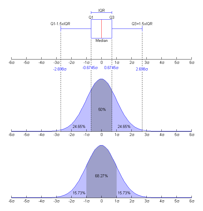
In probability theory, a probability density function (PDF), or density of a continuous random variable, is a function that describes the relative likelihood for this random variable to take on a given value.

The area under the curve of a density is 1 i.e. 100%.

Say you have observations \( (x_1, \ldots, x_n) \) of some continuous random variable. Example the Old Faithful geyser in Yellowstone National Park eruption times

  [1] 3.600 1.800 3.333 2.283 4.533
  [6] 2.883 4.700 3.600 1.950 4.350
 [11] 1.833 3.917 4.200 1.750 4.700
 [16] 2.167 1.750 4.800 1.600 4.250
 [21] 1.800 1.750 3.450 3.067 4.533
 [26] 3.600 1.967 4.083 3.850 4.433
 [31] 4.300 4.467 3.367 4.033 3.833
 [36] 2.017 1.867 4.833 1.833 4.783
 [41] 4.350 1.883 4.567 1.750 4.533
 [46] 3.317 3.833 2.100 4.633 2.000
 [51] 4.800 4.716 1.833 4.833 1.733
 [56] 4.883 3.717 1.667 4.567 4.317
 [61] 2.233 4.500 1.750 4.800 1.817
 [66] 4.400 4.167 4.700 2.067 4.700
 [71] 4.033 1.967 4.500 4.000 1.983
 [76] 5.067 2.017 4.567 3.883 3.600
 [81] 4.133 4.333 4.100 2.633 4.067
 [86] 4.933 3.950 4.517 2.167 4.000
 [91] 2.200 4.333 1.867 4.817 1.833
 [96] 4.300 4.667 3.750 1.867 4.900
[101] 2.483 4.367 2.100 4.500 4.050
[106] 1.867 4.700 1.783 4.850 3.683
[111] 4.733 2.300 4.900 4.417 1.700
[116] 4.633 2.317 4.600 1.817 4.417
[121] 2.617 4.067 4.250 1.967 4.600
[126] 3.767 1.917 4.500 2.267 4.650
[131] 1.867 4.167 2.800 4.333 1.833
[136] 4.383 1.883 4.933 2.033 3.733
[141] 4.233 2.233 4.533 4.817 4.333
[146] 1.983 4.633 2.017 5.100 1.800
[151] 5.033 4.000 2.400 4.600 3.567
[156] 4.000 4.500 4.083 1.800 3.967
[161] 2.200 4.150 2.000 3.833 3.500
[166] 4.583 2.367 5.000 1.933 4.617
[171] 1.917 2.083 4.583 3.333 4.167
[176] 4.333 4.500 2.417 4.000 4.167
[181] 1.883 4.583 4.250 3.767 2.033
[186] 4.433 4.083 1.833 4.417 2.183
[191] 4.800 1.833 4.800 4.100 3.966
[196] 4.233 3.500 4.366 2.250 4.667
[201] 2.100 4.350 4.133 1.867 4.600
[206] 1.783 4.367 3.850 1.933 4.500
[211] 2.383 4.700 1.867 3.833 3.417
[216] 4.233 2.400 4.800 2.000 4.150
[221] 1.867 4.267 1.750 4.483 4.000
[226] 4.117 4.083 4.267 3.917 4.550
[231] 4.083 2.417 4.183 2.217 4.450
[236] 1.883 1.850 4.283 3.950 2.333
[241] 4.150 2.350 4.933 2.900 4.583
[246] 3.833 2.083 4.367 2.133 4.350
[251] 2.200 4.450 3.567 4.500 4.150
[256] 3.817 3.917 4.450 2.000 4.283
[261] 4.767 4.533 1.850 4.250 1.983
[266] 2.250 4.750 4.117 2.150 4.417
[271] 1.817 4.467

The simplest approximation to \( (x_1, \ldots, x_n) \)'s density is a histogram where on the y-axis we are not representing counts, but rather proportions. i.e. the sum of the area of the boxes is 1.

Density is the more general term for proportion.

For two dimensions, each observation is a pair of points \( (x_i, y_i) \) for \( i=1, \ldots, n \). Now

• Our bins are actually boxes, not intervals
• A histogram for these would require a third dimension sticking out of the page to show the height corresponding to each box

So rather we have concentric circles indicate density. We use the geom_density2d() command on the front of your cheatsheet under two variables.