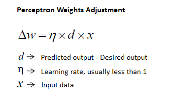
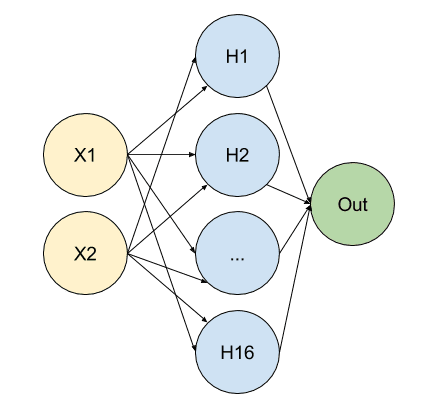
class: title-slide .row[ .col-7[ .title[ # Perceptron ] .subtitle[ ] .author[ ### Laxmikant Soni <br> [Web-Site](https://laxmikants.github.io) <br> [<i class="fab fa-github"></i>](https://github.com/laxmiaknts) [<i class="fab fa-twitter"></i>](https://twitter.com/laxmikantsoni09) ] .affiliation[ ] ] .col-5[ .logo[ <!-- --> ] ] ] --- class: inverse, center, middle # Understanding Perceptron --- class: body # Perceptron <hr> -- .pull-top[ <font size="6"> * A type of neuron having just multiple inputs and one output. * Input is multi-dimensional (i.e. input can be a vector): input x = ( I1, I2, .., In) * Input nodes (or units) are connected (typically fully) to a node (or multiple nodes) in the next layer. * A node in the next layer takes a weighted sum of all its inputs: </font> ] <hr> --- class: body # Example <hr> -- .pull-left[ <font size="6"> Example input x = ( I1, I2, I3) = ( 5, 3.2, 0.1 ) Summed input = 5 w1 + 3.2 w2 + 0.1 w3 </font> ] -- .pull-right[ <!-- --> -- ] <hr> The output node has a "threshold" t. Rule: If summed input ≥ t, then it "fires" (output y = 1). Else (summed input < t) it doesn't fire (output y = 0). --- class: body # Threshold <hr> -- .pull-left[ <font size="6"> The erceptron does not have a priori knowledge, so the initial weights are assigned randomly. SLP sums all the weighted inputs and if the sum is above the threshold (some predetermined value), SLP is said to be activated (output=1). </font> ] -- .pull-right[ <!-- --> -- ] <hr> The input values are presented to the perceptron, and if the predicted output is the same as the desired output, then the performance is considered satisfactory and no changes to the weights are made. However, if the output does not match the desired output, then the weights need to be changed to reduce the error. --- class: body # Algorithm <hr> -- .pull-left[ <!-- --> </font> ] -- .pull-right[ 1. Initialize weights at random 2. For each training pair/pattern (x, ytarget) - Compute output y - Compute error - Use the error to update weights as follows: ∆w = w – wold, ∆w = d * η * x or wnew = wold + ∆w η is called the learning rate or step size and it determines how smoothly the learning process is taking place. d is predicted output - actual output, x input data 3. Repeat 2 until convergence (i.e. error d is zero) ] <hr> --- class: body # Implementing Perceptron for XNOR problem <hr> -- .pull-left[ ```python import numpy as np from keras.models import Sequential from keras.layers.core import Dense ``` ] -- .pull-right[ We import numpy and alias it as np Keras offers two different APIs to construct a model: a functional and a sequential one. We’re using the sequential API hence the second import of Sequential from keras.models. Neural networks consist of different layers where input data flows through and gets transformed on its way. There are a bunch of different layer types available in Keras. These different types of layer help us to model individual kinds of neural nets for various machine learning tasks. In our specific case the Dense layer is what we want. ] <hr> --- class: body # Implementing.. <hr> -- .pull-left[ ```python # the four different states of the XOR gate training_data = np.array([[0,0],[0,1],[1,0],[1,1]], "float32") # the four expected results in the same order target_data = np.array([[0],[1],[1],[0]], "float32") ``` ] -- .pull-right[ We initialize training_data as a two-dimensional array (an array of arrays) where each of the inner arrays has exactly two items. We setup target_data as another two-dimensional array. All the inner arrays in target_data contain just a single item though. Each inner array of training_data relates to its counterpart in target_data. ] <hr> --- class: body # Implementing.. <hr> -- .pull-left[ ```python model = Sequential() model.add(Dense(16, input_dim=2, activation='relu')) model.add(Dense(1, activation='sigmoid')) ``` ] -- .pull-right[ - Sets up an empty model using the Sequential API. - Add a Dense layer to our model in which We set input_dim=2 because each of our input samples is an array of length 2 ([0, 1], [1, 0] etc.). - 16 stand the dimension of the output for this layer. Our model means that we have two input neurons (input_dim=2) spreading into 16 neurons in a so called hidden layer. - Add another layer with an output dimension of 1 and without an explicit input dimension. In this case the input dimension is implicitly bound to be 16 from previous layer. ] <hr> --- class: body # We can visualize our model like this. <hr> -- .pull-top[ <!-- --> ] <hr> --- class: body # Implementing.. <hr> -- .pull-left[ ```python output = activation(input x weight) ``` ] -- .pull-right[ - By setting activation='relu' we specify that we want to use the relu function as the activation function. ] <hr> --- class: body # Implementing.. <hr> -- .pull-left[ ```python model.compile(loss='mean_squared_error', optimizer='adam', metrics=['binary_accuracy']) ``` ] -- .pull-right[ - With neural nets we always want to calculate a number (loss) that tells us how bad our model performs and then try to get that number lower. - mean_squared_error works as our loss function simply because it’s a well proven loss function. - the optimize find the right adjustments for the weights. - last parameter metrics is the binary_accuracy which gives us access to a number that tells us exactly how accurate our predictions are. ] <hr> --- class: body # Implementing.. <hr> -- .pull-left[ ```python model.fit(training_data, target_data, nb_epoch=500, verbose=2) ``` ] -- .pull-right[ - kick off the training by calling model.fit(...) - The first two params are training and target data, - the third one is the number of epochs (learning iterations) - the last one tells keras how much info to print out during the training. ] <hr> --- class: body # Implementing.. <hr> -- .pull-left[ ```python print(model.predict(training_data).round()) ``` ] -- .pull-right[ - Once the training phase finished we can start making predictions. ] <hr> --- class: body # Implementing.. <hr> -- .pull-top[ ```python import numpy as np from keras.models import Sequential from keras.layers.core import Dense # the four different states of the XOR gate training_data = np.array([[0,0],[0,1],[1,0],[1,1]], "float32") # the four expected results in the same order target_data = np.array([[0],[1],[1],[0]], "float32") model = Sequential() model.add(Dense(16, input_dim=2, activation='relu')) model.add(Dense(1, activation='sigmoid')) model.compile(loss='mean_squared_error', optimizer='adam', metrics=['binary_accuracy']) model.fit(training_data, target_data, nb_epoch=100, verbose=2) print(model.predict(training_data).round()) ``` ] <hr> --- class: inverse, center, middle # Thanks