- Selecting variables
- Creating variables
- Updating values
- Subsetting tibbles/data frames
- Aggregation
October 22, 2020
What we learned in the previous class
What we’ll learn today
- Wrap up data processing
- Warm-up exercise
- Pivoting data with
gather()andspread()
- Overview of ggplot2
- Build bar plots + exercise
- Build other plots + exercises
Wrap up data processing
Let’s begin by reading our data
library(tidyverse)
covid <- read_csv('https://rb.gy/lzlylj')
crime <- read_csv('https://rb.gy/5zuayh')
Exercise - 10 minutes
- From the
coviddataset, determine thelocation-monthcombination with the highest number of estimated infections per capita. Exclude dates prior to July and'Global'values inlocation. To do this:Filterrows based on the stated date and locaton conditions- Create a new variable called
infections_per_capitathat reportsest_infectionsoverpopulation - Group by
locationandmonthand suminfections_per_capita - With
arrange, sort byinfections_per_capitaso that rows are in descending (desc()) order
covid %>%
  filter(
    month >= 7 &
    ! location %in% 'Global'
  )
Exercise - 10 minutes
- From the
coviddataset, determine thelocation-monthcombination with the highest number of estimated infections per capita. Exclude dates prior to July and'Global'values inlocation. To do this:Filterrows based on the stated date and locaton conditions- Create a new variable called
infections_per_capitathat reportsest_infectionsoverpopulation - Group by
locationandmonthand suminfections_per_capita - With
arrange, sort byinfections_per_capitaso that rows are in descending (desc()) order
covid %>%
  filter(
    month >= 7 &
    ! location %in% 'Global'
  ) %>%
  mutate(infections_per_capita = est_infections / population)
Exercise - 10 minutes
- From the
coviddataset, determine thelocation-monthcombination with the highest number of estimated infections per capita. Exclude dates prior to July and'Global'values inlocation. To do this:Filterrows based on the stated date and locaton conditions- Create a new variable called
infections_per_capitathat reportsest_infectionsoverpopulation - Group by
locationandmonthand suminfections_per_capita - With
arrange, sort byinfections_per_capitaso that rows are in descending (desc()) order
covid %>%
  filter(
    month >= 7 &
    ! location %in% 'Global'
  ) %>%
  mutate(infections_per_capita = est_infections / population) %>%
  group_by(location, month) %>%
  summarise(infections_per_capita = sum(infections_per_capita, na.rm = TRUE))
Exercise - 10 minutes
covid %>%
  filter(
    month >= 7 &
    ! location %in% 'Global'
  ) %>%
  mutate(infections_per_capita = est_infections / population) %>%
  group_by(location, month) %>%
  summarise(infections_per_capita = sum(infections_per_capita, na.rm = TRUE)) %>%
  arrange(desc(infections_per_capita)) %>%
  head()
## # A tibble: 6 x 3
## # Groups:   location [4]
##   location    month infections_per_capita
##   <chr>       <dbl>                 <dbl>
## 1 Manipur        12                 0.167
## 2 Meghalaya      12                 0.147
## 3 Malta          11                 0.135
## 4 Malta          12                 0.127
## 5 West Bengal    12                 0.107
## 6 Manipur        11                 0.106
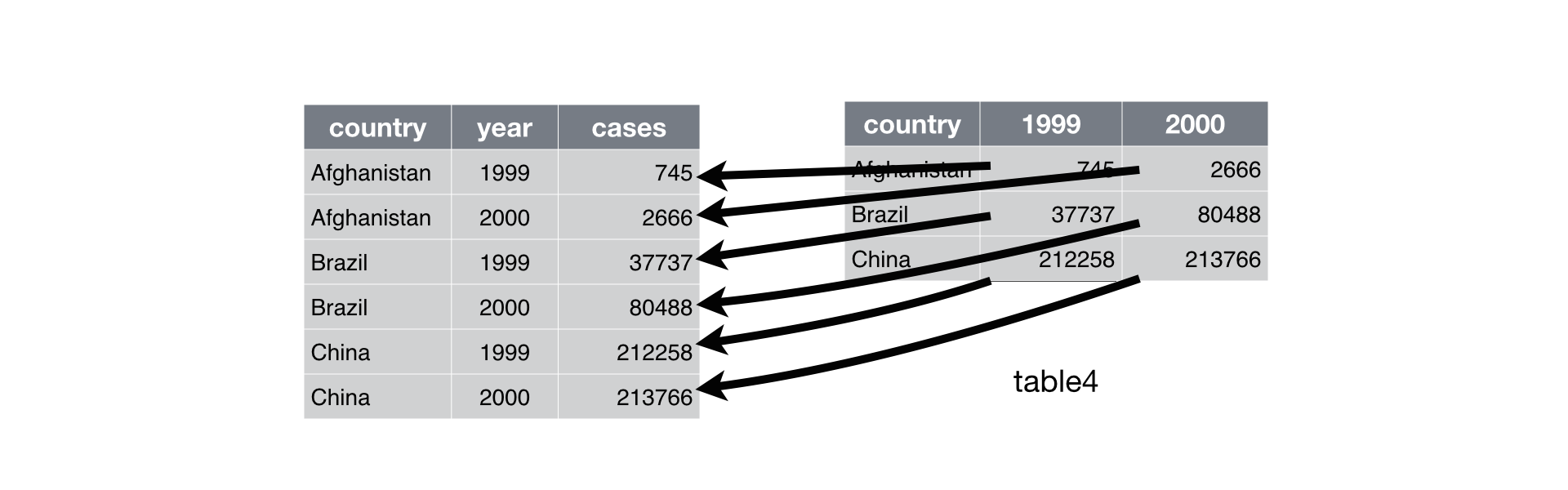
Reshape tibbles
gather()andspread()are the functions we use to reshape (or pivot) data- Reshape means to convert…
- Columns into rows (with
gather()) - Rows into columns (with
spread())
- Columns into rows (with
Reshape tibbles
gather()andspread()are the functions we use to reshape data- Reshape means to convert…
- Columns into rows (with
gather()) - Rows into columns (with
spread())
- Columns into rows (with
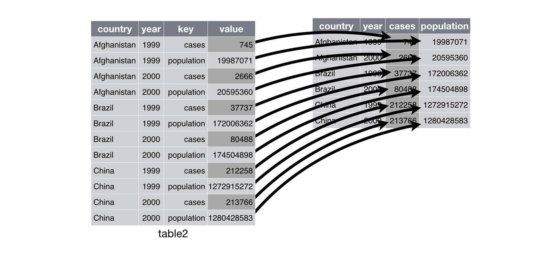
Reshape tibbles
gather()- Convert columns into rows
- Arguments
- Tibble
- Name of column for column names
- Name of column for values in columns
- Which columns you want turn into rows
crime %>%
  select(report_number, occurred_date, reported_date) %>%
  gather(year_type, year, c(occurred_date, reported_date))
Reshape tibbles
gather()- Convert columns into rows
- Arguments
- Tibble
- Name of column for column names
- Name of column for values in columns
- Which columns you want turn into rows
crime %>%
  select(report_number, occurred_date, reported_date) %>%
  gather(year_type, year, 2:3)
Reshape tibbles
crime %>%
  tail(2) %>%
  select(report_number, occurred_date, reported_date) %>%
  gather(year_type, year, c(occurred_date, reported_date))
## # A tibble: 4 x 3
##   report_number year_type     year
##   <chr>         <chr>         <date>
## 1 2010-044880   occurred_date 2010-02-06
## 2 2020-218244   occurred_date 2020-07-20
## 3 2010-044880   reported_date 2010-02-08
## 4 2020-218244   reported_date 2020-07-20
Reshape tibbles
spread()- Convert rows into columns
- Arguments
- Tibble
- Name of column that contains the names of the new columns
- Name of columns that contains the values of the new columns
covid %>%
  filter(! mobility_data_type %in% NA & location %in% c('Peru', 'Ecuador', 'Colombia')) %>%
  group_by(mobility_data_type, location) %>%
  summarise(mobility_composite = mean(mobility_composite, na.rm = TRUE)) %>%
  spread(location, mobility_composite)
Reshape tibbles
covid %>%
  filter(! mobility_data_type %in% NA & location %in% c('Peru', 'Ecuador', 'Colombia')) %>%
  group_by(mobility_data_type, location) %>%
  summarise(mobility_composite = mean(mobility_composite, na.rm = TRUE)) %>%
  spread(location, mobility_composite)
## # A tibble: 2 x 4
## # Groups:   mobility_data_type [2]
##   mobility_data_type Colombia Ecuador  Peru
##   <chr>                 <dbl>   <dbl> <dbl>
## 1 observed              -38.7   -51.1 -54.6
## 2 projected             -12.8   -38.7 -44.0
Reshape tibbles
Exercise #1 - 3 minutes
- With
crime, usegather()to convertprecinct,beat, andneighborhoodcolumns into rows- Name the two new columns whatever you would like
- Keep only the columns you created and
report_number
- Name the two new columns whatever you would like
Exercise #2 - 5 minutes
- With
crime, report the number of incidents byoffense_parent_groupandprecinct. To do this…- First, count incidents with
group_by()andsummarise() - Second, use
spread()to turnprecinctinto columns with counts of incidents
- First, count incidents with
Exercise #1 - 3 minutes
- With
crime, usegather()to convertprecinct,beat, andneighborhoodcolumns into rows- Name the two new columns whatever you would like
- Keep only the columns you created and
report_number
- Name the two new columns whatever you would like
crime %>%
  gather(group, value, c(precinct, beat, neighborhood)) %>%
  select(report_number, group, value) %>%
  sample_n(8)
## # A tibble: 8 x 3
##   report_number group        value
##   <chr>         <chr>        <chr>
## 1 2019-119558   neighborhood <NA>
## 2 2010-214293   neighborhood ALASKA JUNCTION
## 3 2020-236131   precinct     South
## 4 2012-903035   neighborhood GREENWOOD
## 5 2012-099379   precinct     UNKNOWN
## 6 2015-150623   beat         R3
## 7 2012-397750   precinct     North
## 8 2015-240127   precinct     West
Exercise #2 - 5 minutes
- With
crime, report the number of incidents byoffense_parent_groupandprecinct. To do this…- First, count incidents with
group_by()andsummarise() - Second, use
spread()to turnprecinctinto columns with counts of incidents
- First, count incidents with
crime %>%
  filter(! precinct %in% c('UNKNOWN', NA)) %>%
  group_by(precinct, offense_parent_group) %>%
  summarise(n = n())
Exercise #2 - 5 minutes
- With
crime, report the number of incidents byoffense_parent_groupandprecinct. To do this…- First, count incidents with
group_by()andsummarise() - Second, use
spread()to turnprecinctinto columns with counts of incidents
- First, count incidents with
crime %>%
  filter(! precinct %in% c('UNKNOWN', NA)) %>%
  group_by(precinct, offense_parent_group) %>%
  summarise(n = n()) %>%
  spread(precinct, n)
## # A tibble: 32 x 6
##    offense_parent_group                      East North South Southwest  West
##    <chr>                                    <int> <int> <int>     <int> <int>
##  1 ANIMAL CRUELTY                               1     3     1        NA     3
##  2 ARSON                                       26    67    33        19    33
##  3 ASSAULT OFFENSES                          2979  4488  2887      1882  4777
##  4 BAD CHECKS                                 146   321   135        90   213
##  5 BRIBERY                                      1     2     1        NA    NA
##  6 BURGLARY/BREAKING&ENTERING                2054  4898  2135      1396  2618
##  7 COUNTERFEITING/FORGERY                     114   261    89        59   165
##  8 CURFEW/LOITERING/VAGRANCY VIOLATIONS        12     8     8         4    91
##  9 DESTRUCTION/DAMAGE/VANDALISM OF PROPERTY  1845  3489  1871      1355  2459
## 10 DRIVING UNDER THE INFLUENCE                405   663   357       256   564
## # … with 22 more rows
Visualization with ggplot2
ggplot2
- Yardstick for plotting data in R
tidyversepackage- Virtually no limits to plot types
- Plotting resources
Plot types

Plot types

Plot types

Plot types
What we will learn


Requests to learn another plot type?
Plot types
1 discrete variable (plus other optional discrete and/or continuous variables)
1 continuous variable
Plot types
2 continuous variables
1 continuous variable + date variable
Let’s make sure you’re able to plot your data
library(tidyverse)
mpg %>% ggplot() + geom_point(aes(displ, hwy))

Let’s make sure you’re able to plot your data
- If you see a plot, you’re ready to go!
- If you do not, reinstall
tidyverseand re-run the test code
install.packages('tidyverse')
library(tidyverse)
mpg %>% ggplot(aes(displ, hwy))) + geom_point()
- If it still didn’t work, install
ggplot2and re-run the test code
install.packages('ggplot2')
library(ggplot2)
mpg %>% ggplot(aes(displ, hwy)) + geom_point()
How to plot data
- Pick your data
- Pick your chart type (Geom)
- Program stuff like chart titles, axis names, axis types, and legends (Scales)
- Make it pretty (Themes)
- Keep tuning and reuse code
ggplot basics
Geoms
- Every plot needs a
ggplot()function and a geom layer - Separate layers and other plotting functions with
+
ggplot() + geom_bar()       # create bar and stacked bar plots
ggplot() + geom_histogram() # create histograms
ggplot() + geom_point()     # create scatter plots
ggplot() + geom_line()      # create line plots
- Your data is an argument in the
ggplot()function
covid %>% ggplot() + geom_bar()
ggplot(covid) + geom_bar()
Geoms
- Map your data to the plot with
aes()aes()indicates the variables that affect the chart aestheticsaes()can be an argument inggplot()or the geom- Many arguments in the
aes()function aes()arguments reference variables in your tibble
covid %>% ggplot(aes(mobility_data_type)) + geom_bar()
covid %>% ggplot() + geom_bar(aes(mobility_data_type))
aes(x = NULL, y = NULL, color = NULL
  , fill = NULL, alpha = NULL, label = NULL
  , shape = NULL, size = NULL, group = NULL
  , linetype = NULL
  )
Geoms
covid %>% ggplot(aes(x = mobility_data_type)) + geom_bar()
covid %>% ggplot() + geom_bar(aes(x = mobility_data_type))

Geoms
covid %>% ggplot(aes(x = mobility_data_type, fill = mobility_data_type)) + geom_bar()

Geoms
covid %>% ggplot(aes(x = mobility_data_type, fill = as.character(month))) + geom_bar()

Exercise - 7 minutes
- Build a bar chart with
crimedata that shows how many incidents occurred inbeat - Only include these
beatvalues:c('B3', 'E3', 'D2', 'R2', 'O1', 'C3', 'K3') - Color the bars using
offense - Only include these
offensevalues:c('Impersonation', 'Driving Under the Influence', 'Pocket-picking', 'Embezzlement')
Hint
# Use to include/exclude values
filter()
Exercise - 7 minutes
- Build a bar chart with
crimedata that shows how many incidents occurred inbeat - Only include these
beatvalues:c('B3', 'E3', 'D2', 'R2', 'O1', 'C3', 'K3') - Color the bars using
offense - Only include these
offensevalues:c('Impersonation', 'Driving Under the Influence', 'Pocket-picking', 'Embezzlement')
Hint
crime %>%
  filter() %>%
  ggplot()
Exercise - 7 minutes
crime %>%
  filter(
    beat %in% c('B3', 'E3', 'D2', 'R2', 'O1', 'C3', 'K3') &
    offense %in% c('Impersonation', 'Driving Under the Influence'
                  , 'Pocket-picking', 'Embezzlement')
    ) %>%
  ggplot(aes(beat, fill = offense)) +
  geom_bar()

Scales
Axis, legend, and chart titles
Axis names
- Keep names short-ish
- Consider including units in axis name
- It is possible you don’t need an axis name
2 options
# Option 1
labs(x = 'X Axis Title', y = 'Y Axis Title')

# Option 2
xlab('X Axis Title')
ylab('Y Axis Title')
Axis, legend, and chart titles
covid %>%
  filter(! mobility_data_type %in% NA) %>%
  ggplot(aes(x = mobility_data_type, fill = mobility_data_type)) +
  geom_bar() +
  labs(x = 'Mobility Data Type', y = 'Observations (#)')

Axis, legend, and chart titles
Try adding axis names to the beat plot you made during the exercise
crime %>%
  filter(
    beat %in% c('B3', 'E3', 'D2', 'R2', 'O1', 'C3', 'K3') &
    offense %in% c('Impersonation', 'Driving Under the Influence'
                  , 'Pocket-picking', 'Embezzlement')
    ) %>%
  ggplot(aes(beat, fill = offense)) +
  geom_bar() +
  labs(x = 'Seattle Beats', y = 'Incidents by Offense\nClearance Group (#)')

Axis, legend, and chart titles
Legend names
- Keep names short
- Be mindful of what the legend is for
- Color? Fill? Size? etc.
- Consider hiding the legend title for a clean look
labs(fill = '')
labs(fill = element_blank())
labs(fill = NULL)
labs(colour = 'Check out these colors')
Axis, legend, and chart titles
covid %>%
  filter(! mobility_data_type %in% NA) %>%
  ggplot(aes(x = mobility_data_type, fill = mobility_data_type)) +
  geom_bar() +
  labs(x = 'Mobility Data Type', y = 'Observations (#)', fill = 'Check out these colors')

Axis, legend, and chart titles
Try removing the legend name from your beat plot

Axis, legend, and chart titles
Try removing the legend name from your beat plot
crime %>%
  filter(
    beat %in% c('B3', 'E3', 'D2', 'R2', 'O1', 'C3', 'K3') &
    offense %in% c('Impersonation', 'Driving Under the Influence'
                  , 'Pocket-picking', 'Embezzlement')
    ) %>%
  ggplot(aes(beat, fill = offense)) +
  geom_bar() +
  labs(
    x = 'Seattle Beats'
    , y = 'Incidents by Offense\nClearance Group (#)'
    , fill = element_blank()
    )
Axis, legend, and chart titles
Chart titles and subtitles
- Consider making titles (or subtitles) descriptive
- Don’t over use subtitles
# Option 1
labs(title = NULL, subtitle = NULL)

# Option 2
ggtitle(title = NULL, subtitle = NULL)
Axis, legend, and chart titles
covid %>%
  filter(! mobility_data_type %in% NA) %>%
  ggplot(aes(x = mobility_data_type, fill = mobility_data_type)) +
  geom_bar() +
  labs(
    x          = 'Mobility Data Type'
    , y        = 'Observations (#)'
    , fill     = element_blank()
    , title    = '2020 Covid-19 Mobility Types'
    , subtitle = 'Nearly two-thirds of mobility data are observed'
    )
Axis, legend, and chart titles

Axis, legend, and chart titles
Try adding a title to the beat plot

Axis, legend, and chart titles
Try adding a title to the beat plot
crime %>%
  filter(
    beat %in% c('B3', 'E3', 'D2', 'R2', 'O1', 'C3', 'K3') &
    offense %in% c('Impersonation', 'Driving Under the Influence'
                  , 'Pocket-picking', 'Embezzlement')
    ) %>%
  ggplot(aes(beat, fill = offense)) +
  geom_bar() +
  labs(
  x = 'Seattle Beats'
  , y = 'Incidents by Offense\nClearance Group (#)'
  , fill = element_blank()
  , title = 'An Amazing Title'
  )
Axis units
- Change axis units
- This is a good idea and you should do it when its relevant
- Good for x and y axes
install.packages('scales')
library(scales)

scale_y_continuous(labels = percent) # Add a percentage sign to numbers on axis
scale_y_continuous(labels = dollar)  # Add a dollar sign to numbers on axis
scale_y_continuous(labels = comma)   # Add a comma to numbers on axis
Axis units
covid %>%
  filter(! mobility_data_type %in% NA) %>%
  ggplot(aes(x = mobility_data_type, fill = mobility_data_type)) +
  geom_bar() +
  labs(
    x          = 'Mobility Data Type'
    , y        = 'Observations (#)'
    , fill     = element_blank()
    , title    = '2020 Covid-19 Mobility Types'
    , subtitle = 'Nearly two-thirds of mobility data are observed'
    ) +
  scale_y_continuous(labels = comma)
Axis units

Themes
Themes
- Change layer and background colors
- Change fonts
- Change plot borders/boundaries and ticks
- Pre-built themes vs. custom themes
ggplot2themesggthemesthemes
install.packages('ggthemes')
library(ggthemes)
Pre-built themes
Selected ggplot2 themes
theme_classic()
theme_minimal()
theme_dark()
Selected ggthemes themes
theme_stata() + scale_colour_stata() # scale_fill_stata()
theme_economist() + scale_colour_economist() # scale_fill_economist()
theme_fivethirtyeight() + scale_color_fivethirtyeight() # scale_fill_fivethirtyeight()
theme_wsj() + scale_colour_wsj() # scale_fill_wsj()
theme_pander() + scale_colour_pander() # scale_fill_pander()
theme_hc(bgcolor = "darkunica") + scale_colour_hc("darkunica") # scale_fill_hc("darkunica")
Pre-built themes
covid %>%
  filter(! mobility_data_type %in% NA) %>%
  ggplot(aes(x = mobility_data_type, fill = mobility_data_type)) +
  geom_bar() +
  labs(
    x          = 'Mobility Data Type'
    , y        = 'Observations (#)'
    , fill     = element_blank()
    , title    = '2020 Covid-19 Mobility Types'
    , subtitle = 'Nearly two-thirds of mobility data are observed'
    ) +
  scale_y_continuous(labels = comma) +
  theme_economist() +
  scale_fill_economist()
Pre-built themes
Economist theme

Pre-built themes

Pre-built themes
Try adding a theme to the beat plot

Custom themes
- You can create custom themes with
theme() - Greater control over chart aesthestics
- Use custom themes in place of pre-built themes if pre-built themes don’t cut it
- Also, use custom themes to augment pre-built themes
Custom themes
theme(
  plot.title         = element_text(size=14, face="bold", vjust=1)
  , plot.background  = element_blank()
  , panel.grid.major = element_blank()
  , panel.grid.minor = element_blank()
  , panel.border     = element_blank()
  , panel.background = element_blank()
  , axis.ticks       = element_blank()
  , axis.text        = element_text(colour="black", size=12)
  , axis.text.x      = element_text(angle=45, hjust=1)
  , legend.title     = element_blank()
  , legend.position  = "none"
  , legend.text      = element_text(size=12)
  )
Exercise - 5 minutes
We answered the two questions below in the previous class. How would you turn the tabular output data into a chart?
- In
covid, whichlocationreports the largest number of estimated infections in September, excluding'Global'values? - In
crime, of all'ASSAULT OFFENSES'values inoffense_parent_groupwhichoffensevalue has the fewest incidents?
covid %>%
  group_by(month, location) %>%
  summarise(est_infections = sum(est_infections, na.rm = TRUE)) %>%
  filter(month %in% 9 & ! location %in% 'Global') %>%
  arrange(desc(est_infections)) %>%
  head()
Exercise - 5 minutes
How would you turn the tabular output data into a chart?
covid %>%
  group_by(month, location) %>%
  summarise(est_infections = sum(est_infections, na.rm = TRUE)) %>%
  filter(month %in% 9 & ! location %in% 'Global') %>%
  arrange(desc(est_infections)) %>%
  head() %>%
  ggplot(aes(x = reorder(location, est_infections), y = est_infections, fill = location)) +
  geom_bar(stat = "identity") +
  guides(fill=guide_legend(nrow=3)) +
  labs(x = 'Location', y = 'Estimated Infections (#)') +
  coord_flip() + # coord_flip() is a new function
  ggthemes::theme_hc()
Exercise - 5 minutes
How would you turn the tabular output data into a chart?

Exercise - 5 minutes
How would you turn the tabular output data into a chart?
covid %>%
  group_by(month, location) %>%
  summarise(est_infections = sum(est_infections, na.rm = TRUE)) %>%
  filter(month %in% 9 & ! location %in% 'Global') %>%
  arrange(desc(est_infections)) %>%
  head() %>%
  ggplot(aes(x = reorder(location, est_infections), y = est_infections, fill = location)) +
  geom_bar(stat = "identity") +
  guides(fill=guide_legend(nrow=3)) +
  labs(x = 'Location', y = 'Estimated Infections (#)') +
  coord_flip() + # coord_flip() is a new function
  ggthemes::theme_hc()
New argument and functions
geom_bar(stat = 'identity')       # IMPORTANT: use stat when working with aggregated data
reorder(location, est_infections) # reorder() to sort rows/columns in your visualization
coord_flip()                      # coord_flip(): x becomes y; y becomes x
Exercise - 5 minutes
We answered the two questions below in the previous class. How would you turn the tabular output data into a chart?
- In
covid, whichlocationreports the largest number of estimated infections in September, excluding'Global'values? - In
crime, of all'ASSAULT OFFENSES'values inoffense_parent_groupwhichoffensevalue has the fewest incidents?
crime %>%
  group_by(offense_parent_group, offense) %>%
  summarise(incident = n()) %>%
  filter(offense_parent_group %in% 'ASSAULT OFFENSES' & ! offense %in% NA)
## # A tibble: 3 x 3
## # Groups:   offense_parent_group [1]
##   offense_parent_group offense            incident
##   <chr>                <chr>                 <int>
## 1 ASSAULT OFFENSES     Aggravated Assault     3754
## 2 ASSAULT OFFENSES     Intimidation           3963
## 3 ASSAULT OFFENSES     Simple Assault         9527
Exercise - 5 minutes
How would you turn the tabular output data into a chart?
crime %>%
  group_by(offense_parent_group, offense) %>%
  summarise(incident = n()) %>%
  filter(offense_parent_group %in% 'ASSAULT OFFENSES' & ! offense %in% NA) %>%
  ggplot(aes(reorder(offense, -incident), incident)) +
  geom_bar(stat = 'identity') +
  theme_classic()

Exercise - 15 minutes
- From the
crimedataset, report the mean difference inreported_dateandoccurred_datevalues bybeat.- The variable that tells us the difference between
reported_dateandoccurred_dateshould be calleddate_dif - In your output of mean values by
beatonly report rows where the number ofbeatvalues in the dataset is greater than 3000 - You’ll use
transmuteandfilteras well asgroup_byandsummariseto solve this problem - The dataframe should have three variables:
beat,date_dif,n
- The variable that tells us the difference between
- Create a bar plot that that shows
date_difvalues bybeat
Hint
crime %>%
  transmute(
    beat
    , date_dif = reported_date - occurred_date
  ) %>%
Exercise - 15 minutes
- From the
crimedataset, report the mean difference inreported_dateandoccurred_datevalues bybeat.- The variable that tells us the difference between
reported_dateandoccurred_dateshould be calleddate_dif - In your output of mean values by
beatonly report rows where the number ofbeatvalues in the dataset is greater than 3000 - You’ll use
transmuteandfilteras well asgroup_byandsummariseto solve this problem - The dataframe should have three variables:
beat,date_dif,n
- The variable that tells us the difference between
- Create a bar plot that that shows
date_difvalues bybeat
crime %>%
  transmute(
    beat
    , date_dif = reported_date - occurred_date
  ) %>%
  group_by(beat) %>%
  summarise(
    date_dif = mean(date_dif, na.rm = TRUE)
    , n = n()
  ) %>%
  filter(n > 3000) %>%
Exercise - 15 minutes
crime %>%
  transmute(
    beat
    , date_dif = reported_date - occurred_date
  ) %>%
  group_by(beat) %>%
  summarise(
    date_dif = mean(date_dif, na.rm = TRUE)
    , n = n()
  ) %>%
  filter(n > 3000) %>%
  ggplot(aes(x = beat, y = date_dif)) +
  geom_bar(stat = 'identity')
Exercise - 15 minutes

Exercise - 5 minutes
- Take an extra 5 minutes to do the following
- Add a theme to your plot
- Change the axis names
- Add a plot title
- Arrange the
beatcolumns bydate_dif - Remove
NAbeatvalues
- Add a theme to your plot
Exercise - 5 minutes

Exercise - 5 minutes
crime %>%
  transmute(
    beat
    , date_dif = reported_date - occurred_date
  ) %>%
  group_by(beat) %>%
  summarise(
    date_dif = mean(date_dif, na.rm = TRUE)
    , n = n()
  ) %>%
  filter(n > 3000 & ! beat %in% c(NA, 'UNKNOWN')) %>%
  ggplot(aes(reorder(beat, -date_dif), date_dif)) +
  geom_bar(stat = 'identity') +
  labs(
    y = 'Average delay in reporting (days)'
    , x = 'Beat'
    , title = 'Beat U3 sees the longest delay in events reporting'
    ) +
  theme_classic()
Histograms, scatterplots, and line plots
Histograms: 1 continuous variable
binsis the argument you use to indicate the number of columns in your histogram
covid %>%
  ggplot(aes(mobility_composite)) +
  geom_histogram()

Histograms: 1 continuous variable
binsis the argument you use to indicate the number of columns in your histogram
covid %>%
  ggplot(aes(mobility_composite)) +
  geom_histogram(bins = 10)

Scatterplots: 2 continuous variables
covid %>%
  ggplot(aes(x = deaths_p100k, y = est_infections_p100k)) +
  geom_point()

Scatterplots: 2 continuous variables
covid %>%
  ggplot(aes(x = deaths_p100k, y = est_infections_p100k)) +
  geom_point()
geom_count() # adds a size component to your scatterplot
geom_jitter() # adjusts cartesian location of point relative to other points
Line plot: 1 continuous variable + date variable
covid %>%
  group_by(date) %>%
  summarise(total_tests = sum(total_tests, na.rm = TRUE)) %>%
  ggplot(aes(x = date, y = total_tests)) +
  geom_line(stat = 'identity')

Line plot: 1 continuous variable + date variable
covid %>%
  group_by(date) %>%
  summarise(total_tests = sum(total_tests, na.rm = TRUE)) %>%
  ggplot(aes(x = date, y = cumsum(total_tests))) + # cumsum() is a new function!
  geom_line(stat = 'identity')

Exercise - 5 minutes
- With either dataset,
covidorcrime, create a scatterplot or line plot - Include one
aes()arguments in addition toxandy- For example,
size,shape,colororalpha
- For example,
- Line plots: 1 continuous variable + date variable
- Scatterplot: 2 continuous variables
- Use
group_by()andsummarise()if you would like
 crime %>%
  filter(! precinct %in% NA) %>%
  ggplot(aes(reported_date, occurred_date, color = precinct)) +
  geom_point() +
  theme_classic()
Exercise - 5 minutes
 crime %>%
  filter(! precinct %in% NA) %>%
  ggplot(aes(reported_date, occurred_date, color = precinct)) +
  geom_point() +
  theme_classic()

Exercise - 15 minutes
- Create a plot from the
crimedataset that shows the number of incidents by a character variable (you pick) and a time of day variable that indicates if the incident occurred in the AM or PM (first half or second half of the day)- Create a new variable with
mutate()calledoccurred_time_ampmthat tells whether an incident occurred in the AM or PM. - Make sure your axes are labeled correctly
- Give your chart a title
- Use
occurred_time_ampmin thecolororfillarguments inaes() - Use a pre-built theme
- Create a new variable with
Exercise - 15 minutes

Exercise - 15 minutes
crime %>%
  mutate(occurred_time_ampm = ifelse(occurred_time >= 1200, 'PM', 'AM')) %>%
  filter(
    ! occurred_time_ampm %in% NA &
    ! precinct %in% NA
    ) %>%
  group_by(precinct, occurred_time_ampm) %>%
  summarise(n = n()) %>%
  ungroup %>%
  ggplot(aes(reorder(precinct, n), n, fill = occurred_time_ampm)) +
  geom_bar(stat = 'identity') +
  coord_flip() +
  theme_wsj() +
  scale_fill_wsj() +
  labs(title = 'Most incidents occur\nin the PM', fill = 'Time of Day')