Publication Quality Figures with ggplot2 - Part 1
Ömer Faruk Örsün | omerorsun@nyu.edu
Why do we need figures?
Question
Can you guess the similarity among the following 12 different datasets? 
Answer
They all have the same: 
Preparation
library(ggpubr)
library(ggplot2)
library(stargazer)
#let's load our data
setwd("~/Dropbox/Data Analysis F20 Recitation/Recitation Content/Recitation 4")
Pokemon<-read.csv("Pokemon.csv",header=T,na.strings="?")
#tell R that we are only working with Pokemon dataWe will use Pokemon dataset. The data as described by Myles O’Neill is:
- \(#\): ID for each pokemon
- Name: Name of each pokemon
- Type 1: Each pokemon has a type, this determines weakness/resistance to attacks
- Type 2: Some pokemon are dual type and have 2
- Total: sum of all stats that come after this, a general guide to how strong a pokemon is
- HP: hit points, or health, defines how much damage a pokemon can withstand before fainting
- Attack: the base modifier for normal attacks (eg. Scratch, Punch)
- Defense: the base damage resistance against normal attacks
- SP Atk: special attack, the base modifier for special attacks (e.g. fire blast, bubble beam)
- SP Def: the base damage resistance against special attacks
- Speed: determines which pokemon attacks first each round
unique(factor(Pokemon$Type.1)) ## [1] Grass Fire Water Bug Normal Poison Electric Ground
## [9] Fairy Fighting Psychic Rock Ghost Ice Dragon Dark
## [17] Steel Flying
## 18 Levels: Bug Dark Dragon Electric Fairy Fighting Fire Flying Ghost ... WaterThe Grammar of Graphics
A graph consists of several components:
Data
The data element is the data set itself. ggplot doesnt accept matrices, lists etc. The data you want to graph should be in a dataframe. Let’s initialize our graph, then fill it step by step.
stargazer(Pokemon, header=FALSE, type='html', title="Descriptive Statistics",digits=1,
summary.stat=c("n","mean","sd","min","max")
)| Statistic | N | Mean | St. Dev. | Min | Max |
| X. | 800 | 362.8 | 208.3 | 1 | 721 |
| Total | 800 | 435.1 | 120.0 | 180 | 780 |
| HP | 800 | 69.3 | 25.5 | 1 | 255 |
| Attack | 800 | 79.0 | 32.5 | 5 | 190 |
| Defense | 800 | 73.8 | 31.2 | 5 | 230 |
| Sp..Atk | 800 | 72.8 | 32.7 | 10 | 194 |
| Sp..Def | 800 | 71.9 | 27.8 | 20 | 230 |
| Speed | 800 | 68.3 | 29.1 | 5 | 180 |
| Generation | 800 | 3.3 | 1.7 | 1 | 6 |
bestpokemon<-ggplot(data = Pokemon)
bestpokemon
But our axes are not defined We define it by graph’s aesthetics: aes()
Aesthetics: aes()
What will represent the axes on my plot? Beside variables that will represent axes do we want to see some additional information, which can be shown by different shapes, colors, sizes?
bestpokemon<-ggplot(data = Pokemon)+aes(x = Attack, y = Defense)
bestpokemon
The axes are set but we dont have anything in it. We should choose our geometrical shapes geom()
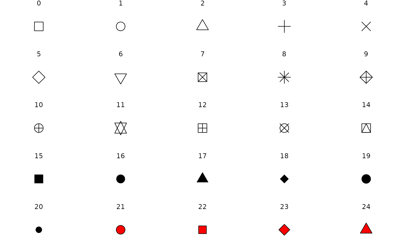
Geometrical Shapes: geom_()
Geometric objects are the actual marks we put on a plot. Examples include:
- points (
geom_point(), for scatter plots, dot plots, etc) - lines (
geom_line(), for time series, trend lines, etc) - boxplot (
geom_boxplot(), for, well, boxplots!)
A plot must have at least one geom; there is no upper limit. You can add a geom to a plot using the + operator
You can get a list of available geometric objects in this CHEATSHEET first and then more details with the following command:
help.search("geom_", package = "ggplot2")Continuous Y and Continuous X
Let’s create a scatter plot!
bestpokemon<-ggplot(data = Pokemon)+
aes(x = Attack, y = Defense)+
geom_point()
bestpokemon
Now we can see the distribution of attack and defense power of different pokemons.
We can play with the shape with shape =, size of the dots with size =, the transparency with alpha= the color as color =:
bestpokemon<-ggplot(data = Pokemon)+
aes(x = Attack, y = Defense)+
geom_point(shape = 17, size = 1, alpha=0.75, color = "blue")
bestpokemon
Let’s make it more interesting: Let’s define
- the color based on whether a pokemon is a legendary one,
- shape based on the generation,
- size based on HP.
To do this customization, we use aes() inside geom_point(). You can now see
aes()can be used as separate to define the global settings for our plotaes()can be used ingeom_XXX()asgeom_XXX(aes())to distinguish colors, shapes, etc for the givengeom_XXXbased on a variable.
Let’s see the example code
bestpokemon<-ggplot(data = Pokemon)+
aes(x = Attack, y = Defense)+
geom_point(alpha=0.75,
aes(shape = as.factor(Generation),
color = Legendary,
size = HP
)
)
bestpokemon
If we want to distinguish between legendary and ordinary pokemons and we want the colors to be globally (for both geom_point() and geom_smooth) based on legendary, then we can put everything into aes(x = Attack, y = Defense, color=Legendary)
ggplot(data = Pokemon)+
aes(x = Attack, y = Defense, color=Legendary)+
geom_point()+
geom_smooth()
or by including aes(color=Legendary) into geom_XXX()functions as follows:
ggplot(data = Pokemon)+
aes(x = Attack, y = Defense)+
geom_point(aes(color=Legendary))+
geom_smooth(aes(color=Legendary))
But this does not look as clean as the first one.
Let’s continue with our exercise with different geometries: a rug plot with geom_rug() and set the line to linear regression fit with method="lm" and label things:
bestpokemon<-ggplot(data = Pokemon)+
aes(x = Attack, y = Defense, color=Legendary)+
geom_rug()+
geom_smooth(method="lm")+
labs(title = "My Main Title for Rug Plot ", subtitle = "A subtitle", x = "Defense Score", y="Attack Score", color="Is the Pokemon Legendary?")
bestpokemon
Please pay attention to color="Is the Pokemon Legendary?". Because I distinguish the pokemons based on the color, I use color for the labeling. If I used shape, transparency (using alpha), or the fill, then I would have to write, e.g., fill="Is the Pokemon Legendary?". See the example:
bestpokemon<-ggplot(data = Pokemon)+
aes(x = Attack, y = Defense, fill=Legendary)+
geom_rug()+
geom_smooth(method="lm")+
labs(title = "My Main Title for Rug Plot ", subtitle = "A subtitle", x = "Defense Score", y="Attack Score", fill="Is the Pokemon Legendary?")
bestpokemon
If we want to distinguish between different health levels (a continuous variable), then I include it again as a color.
bestpokemon<-ggplot(data = Pokemon)+
aes(x = Attack, y = Defense)+
geom_point(aes(color=HP))
bestpokemon
If the variable had discrete values, I would have to convert it to factor using as.factor() or factor() as in the example we had above. Otherwise, ggplot may assume the variable is continuous and you would not get distinct colors as in the following example:
The following is with factor()
ggplot(data = Pokemon)+
aes(x = Attack, y = Defense)+
geom_point(alpha=0.75, aes(color = factor(Generation)))
The following is without factor()
ggplot(data = Pokemon)+
aes(x = Attack, y = Defense)+
geom_point(alpha=0.75, aes(color = Generation))
Continuous Y and Discrete X
Let’s work with continuous Y and discrete X Geometries:
This is a histogram for continuous variables:
ggplot(data = Pokemon) +
geom_histogram(aes(x = Speed),bin=5)
Density
ggplot(data = Pokemon) +
geom_density(aes(x = Speed), fill="blue", alpha=0.55)
ggplot(data = Pokemon) +
geom_density(aes(x = Speed, fill=Legendary), alpha=0.7)
This is a bar graph for discrete variables:
ggplot(data = Pokemon) +
geom_bar(aes(x = factor(Generation)), color="gray", fill="white")
I want to see different generationss and whether they are legendary or not:
ggplot(data = Pokemon) +
geom_bar(aes(x = factor(Generation), color=Legendary))
Hımm, looks bad. Let’s try fill:
ggplot(data = Pokemon) +
geom_bar(aes(x = factor(Generation), fill=Legendary))
What about histogram of speed for different groups?
ggplot(data = Pokemon) +
geom_histogram(aes(x = Speed, fill=Legendary))
Let’s check if Legendary pokemons have a higher attack score based on their generations:
ggplot(data = Pokemon) +
aes(x = factor(Legendary), y=Attack, fill=factor(Generation))+
geom_boxplot()
We can test whether different legendary pokemons are more likely to be different in attack, defense and health than nonlegendary ones. We create confidence intervals based on our conf.interval()function and test whether they are different or not:
# Our function:
conf.interval = function(x, confint = 0.95){
if(confint==0.95){
stderr = plotrix::std.error(x, na.rm=TRUE)
out = c(mean(x) - 1.96*stderr,
mean(x) + 1.96*stderr)
} else if (confint==0.99) {
stderr = plotrix::std.error(x, na.rm=TRUE)
out = c(mean(x) - 2.575*stderr,
mean(x) + 2.575*stderr)
} else {
stop("confint must be either 0.95 or 0.99")
}
return(out)
}
confint_legendary.attack= conf.interval(Pokemon$Attack[Pokemon$Legendary=="True"], 0.95)
confint_nonlegendary.attack = conf.interval(Pokemon$Attack[Pokemon$Legendary=="False"], 0.95)
confint_legendary.defense = conf.interval(Pokemon$Defense[Pokemon$Legendary=="True"], 0.95)
confint_nonlegendary.defense = conf.interval(Pokemon$Defense[Pokemon$Legendary=="False"], 0.95)
confint_legendary.health = conf.interval(Pokemon$HP[Pokemon$Legendary=="True"], 0.95)
confint_nonlegendary.health = conf.interval(Pokemon$HP[Pokemon$Legendary=="False"], 0.95)
attackdata<-data.frame(Legendary=c("Legendary","Ordinary"),
LCI=c(confint_legendary.attack[1],confint_nonlegendary.attack[1]),
HCI=c(confint_legendary.attack[2],confint_nonlegendary.attack[2]),
mean=c(mean(Pokemon$Attack[Pokemon$Legendary=="True"]),mean(Pokemon$Attack[Pokemon$Legendary=="False"]))
)
defensedata<-data.frame(Legendary=c("Legendary","Ordinary"),
LCI=c(confint_legendary.defense[1],confint_nonlegendary.defense[1]),
HCI=c(confint_legendary.defense[2],confint_nonlegendary.defense[2]),
mean=c(mean(Pokemon$Defense[Pokemon$Legendary=="True"]),mean(Pokemon$Defense[Pokemon$Legendary=="False"]))
)
heatlthdata<-data.frame(Legendary=c("Legendary","Ordinary"),
LCI=c(confint_legendary.health[1],confint_nonlegendary.health[1]),
HCI=c(confint_legendary.health[2],confint_nonlegendary.health[2]),
mean=c(mean(Pokemon$HP[Pokemon$Legendary=="True"]),mean(Pokemon$HP[Pokemon$Legendary=="False"]))
)
attackdata
defensedata
heatlthdata## Legendary LCI HCI mean
## 1 Legendary 109.29907 124.05478 116.67692
## 2 Ordinary 73.46508 77.87369 75.66939## Legendary LCI HCI mean
## 1 Legendary 92.79249 106.53059 99.66154
## 2 Ordinary 69.36080 73.75757 71.55918## Legendary LCI HCI mean
## 1 Legendary 87.45763 98.01930 92.73846
## 2 Ordinary 65.38874 68.97589 67.18231Let’s test our hypothesis using overlaping confidence intervals approach: We use geom_linerange() as our geometry in R:
attackgraph<-ggplot()+
geom_linerange(data = attackdata,
mapping=aes(x=Legendary, ymin=LCI, ymax=HCI),
size=1, color="red"
)+
geom_point(data = attackdata,
mapping=aes(x=Legendary, y=mean),
size=4, shape=21, fill="white"
)+
ylim(60, 130)+
labs(title = "Attack")
ggarrange(attackgraph, defensegraph, healthgraph,
ncol = 3, nrow = 1)
Practice Question 1
Can you reproduce this?
Question

Answer
ggplot(data = Pokemon)+
aes(x = factor(Generation), y =Speed)+
geom_point(aes(color=HP))+
labs(title="Distribution of Speed across Different Generations", x="Generation", y="Speed of Pokemon", color="Health")
Can we improve interpretability of this? We dont see how the data is distributed. Hint: use geom_jitter()
Improve by geom_jitter()
geom_jitter randomly moves points from the x axis so that we can see
ggplot(data = Pokemon)+
aes(x = factor(Generation), y =Speed)+
geom_jitter(aes(color=HP), size=0.3)+
labs(title="Distribution of Speed across Different Generations", x="Generation", y="Speed of Pokemon", color="Health")
Practice Question 2
Can you reproduce this?
Question
Can you reproduce this.
Hint: Bar graphs can have position="stack" (default value), position="dodge". If you want proportions, rather than counts, use position="fill".

Answer
ggplot(data=Pokemon)+aes(x=factor(Generation), fill=Legendary)+
geom_bar(position="dodge")