Reproducible Research

Christopher J. Mecklin
Department of Mathematics & Statistics
Biology and Mathematics in Population Studies,BioMaPS 2
Murray State University
May 29-30, 2013
www.rpubs.com/cmecklin/Workshop

An outline for the two afternoons

Day One

• Introduction to Reproducible Research (RR)
• Reasons for RR
• Tools for RR

Day Two

• Statistical Graphics
• Creating a Reproducible Report

• Donald Knuth(Literate Programming) Instead of imagining that our main task is to instruct a computer what to do, let us concentrate rather on explaining to human beings what we want a computer to do. (Knuth is a legend in computer science and wrote this in 1984!)

• Jon Claerbout The principal goal of scientific publications is to teach new concepts, show the resulting implications of those concepts in an illustration, and provide enough detail to make the work reproducible. (Claerbout is a well-known geophysicist and he said this in 1992!)

• RRPlanet.com Reproducible research refers to the idea that the ultimate product of research is the paper along with the full computational environment used to produce the results in the paper such as the code, data, etc. necessary for reproduction of the results and building upon the research.

• ReproducibleResearch.net After a colleague asked something about a paper you wrote, you spend a considerable amount of time finding back the right program files you used in that paper. Not to talk about the time to get back to the set of parameters used to produce that nice result. This is some motivation for why you want to do reproducible research.

Professor Jon Claerbout, Stanford

• An article about computational science in a scientific publication is not the scholarship itself, it is merely advertising of the scholarship.

• The actual scholarship is the complete software development environment and the complete set of instructions which generated the figures.

• Robert Gentleman

  Given:

  1. a data set (which is where most scientific papers start)
  2. a description of the analysis that leads to the figures and tables
  3. Can a reasonably competent individual reproduce the results?
     

• David Donoho

  • Traditional scientific publication is incapable of finding and rooting out errors in scientific computation; this must be recognized as a crisis. Reproducible computational research, in which the full computational environment that produces a result is published along with the article, is an important recent development, and a necessary response to this crisis.

Right now I am in the process of writing a paper with Dr. Kate He, her student Jie Yang, and last year's BioMaPS team of Sam Pellock and Andrew Thompson.

This paper is dealing the validity of Darwin's Naturalization Hypothesis and utilizes a database of plant species found in Kentucky compiled by Pellock, Thompson, and Yang.

My main role in the project was providing Sam & Andrew with help in the intial data analyses, such as what was presented on their NIMBioS poster, and then doing more sophisticated data analyses for the final paper.

I will be the first to admit that I did not fully follow the protocol for reproducible research as I'll be talking about. I'm still fairly new to the concept.

Over the past few months, Dr. He and myself have had a exchange of emails that I suspect are very similar to thousands of such exchanges between biologists (and other scientists) and statistician/mathematicians.

This exchange has included me having to track down a data file that I no longer had, but fortunately Andrew still had it and loaded onto Google Docs.

Our manuscript was recently submitted and reviewed. Our manuscript does not include access to the raw data or the code for my statistical analyses, so the referee would not be able to reproduce my analyses.

I must admit that there was an error in my analyses (I had the wrong df for a variable) that the referee did spot. While it was an embarassing faux pas, I've been able to correct the statistics and Dr. He has made slight revisions to the discussion.

What if the referee did not catch this error? What if the error was such that it would have been impossible to detect in a non-reproducible document???

• Are you convinced that we, as scientists, should go through the trouble of producing reproducible research?

• Should we provide our data and our methodology and make it easier for others to replicate our findings?

• The keynote address at the International R Users Conference in Nashville in 2012 was delivered by Dr. Kevin R. Coombes, from The University of Texas M. D. Anderson Cancer Center in Houston (the man with beard & ponytail in the 60 Minutes clips)

• Dr. Coombes says the term reproducible research on the web extra clip, but it wasn't defined for the viewer.

• He and Dr. Keith Baggerly used forensic bioinformatics to uncover not just mistakes, but fraud, in the work done at Duke by Dr. Anil Potti

• This might not be as sexy as the forensic work you see on popular TV shows, but this is the real power of biomathematics at work.

• Discuss the video clips

• Why would researchers like Dr. Potti commit such fraud?

• What can be done to prevent future such occurences?

• Has your views on reproducible research been affected after watching the Deception at Duke clip?

• Keith Baggerly The most common mistakes are simple. This simplicity is often hidden. The most simple mistakes are common.

• Kevin Coombes As a result of our efforts, four clinical trials have been terminated and at least eight papers have been retracted. (Baggerly & Coombes spent approx. 2000 hours on this matter.)

• Baggerly-Coombes Paper One theme that emerges is that the most common errors are simple; conversely, it is our experience that the most simple errors are common.

• Brad Carlin Reproducibility in research is extremely important!! Given the data and the analysis details/code, others should be able to generate the same findings.

• Andrew Gelman This is horrible! But, in a way, it's not surprising. I make big mistakes in my applied work all the time. I mean, all the time...(Mecklin: Me too!)...Genetics, though, seems like more of a black box...operating some of these methods seems like knitting a sweater inside a black box: it's a lot harder to notice your mistakes if you can't see what you're doing, and it can be difficult to tell by feel if you even have a functioning sweater when you're done with it all.

• It does seem kinda funny that the American Cancer Society took away their [Duke's] grant because of a false statement on a resume. It's a bit like jailing Al Capone on tax evasion, I guess.

• Wikipedia After leaving Duke, Potti hired Online Reputation Manager, a reputation management company, to improve search results for his name.

• Nature/Keith Baggerly Journals should demand that authors submit sufficient detail for the independent assessment of their paper's conclusions...we owe it to patients and to the public to do what we can to ensure the validity of the research we publish.

• New York Times "Our intuition is pretty darn poor," Dr. Baggerly said.

• The Economist The whole thing, then, is a mess. Who will carry the can remains to be seen. But the episode does serve as a timely reminder of one thing that is sometimes forgotten. Scientists are human, too.

• Victoria Stodden

Other branches of science incorporate reproducibility of results.

• deductive branch (mathematics, formal logic): the well-defined concept of the proof

• inductive branch (experimental sciences): machinery of hypothesis testing, structured communication of methods and protocols.

• Computational Science must develop standards for reproducibility before it can be considered a third branch of the scientific method.

I will come at this from the standpoint of statistical computing. Mathematicians would probably use MATLAB or similar instead.

• Statistical Software Packages
  • SAS
    
  • SPSS
    
  • Other commerical packages (Minitab, STATA, etc.)
    
  • R (open source statistical programming language)
    
  • Other free stats packages (WinBUGS, MARK, others)

What do you do?

• response

• response

• response

(Responses included "email Mecklin", "use my calcalator", "use SAS", "use R")

Here's how applied statistics worked at the University of Northern Colorado in the late twentieth century...

• We had SAS. When I first started grad school it was still only available on the mainframe, but shortly after learning the arcane ways of VAX/VMS, we got it on desktop PCs. (No, I have never used punchcards!)

• My advisor taught applied statistics courses to grad students in psychology and education. He taught them how to write SAS code.

• They hated it!

• Often these students would go ahead and analyze their data for their dissertations or other projects with programs such as SPSS.

• They hated SPSS less because it had menus and you could click and create tons of graphs and reams of output.

• Someone hired me once to help them run their stats and I got to use SPSS. Of course, I was just running through menus and clicking boxes and you asked me to reproduce that analysis today, I couldn't.

• I still have a box of 3.5 inch floppies with SAS programs from my dissertation and other projects. I could reproduce those analyses today

• Well, maybe not. I don't have a floppy drive anymore!

• RCommander (the leading GUI, based on the Rcmdr package)

• RStudio (the leading IDE)

• R Markdown (what you can use to write reproducible reports and process in various ways)

• LaTeX (typesetting program that mathematicians/statisticians all know)

• Sweave and knitr (integrate your R code/results into your LaTeX document )

• slidify (to make the HTML5 slide deck as an alternative to PowerPoint or "beamer")

• RPubs (a way to publish your RMarkdown and RPresentation documents online)

Not meant as an exhaustive tutorial...

• R Studio: Workspace...Import Dataset

URL: http://campus.murraystate.edu/academic/faculty/cmecklin/snappingturtle.txt

• R console: read.table, read.csv, others

• R Commander:

  • Data...New data set. Invokes R's Data Editor (yuck)
  • Data...Import data. Can import from:
  • .txt and .csv files
  • EXCEL files (unless you own a Mac)
  • SAS/SPSS/STATA/Minitab

Suppose we are trying to estimate what percentage of the continental U.S. (no Alaska or Hawaii) is roadless, i.e. no roads within a 1 mile radius. I don't know what this percentage is. We need to...

• form a hypothesis

• collect data

• store data

• graph data(we'll worry about tomorrow)

• analyze data

• create a report to share our results

Let's form a hypothesis for Nick Horton's roadless activity.

If we are classically trained freqentists, we'll probably write a null hypothesis and an alternative hypothesis.

If we are Bayesian, we'll think about what sort of prior distribution and likelihood to use.

You will need to type the following command into the R console.

source("http://www.math.smith.edu/~nhorton/roadless.R")

You can go to Horton's link to see his R code.

Let's display the first 20 locations that were generated

myroadless

##    sample latitude longitude withincontinent within1mile location notes
## 1       1    27.25    -90.89              NA          NA               
## 2       2    35.13   -113.70              NA          NA               
## 3       3    44.06   -116.51              NA          NA               
## 4       4    41.74    -97.40              NA          NA               
## 5       5    39.24    -70.92              NA          NA               
## 6       6    35.78    -89.76              NA          NA               
## 7       7    34.58    -70.27              NA          NA               
## 8       8    33.53    -87.54              NA          NA               
## 9       9    47.15    -77.91              NA          NA               
## 10     10    35.21    -65.55              NA          NA               
## 11     11    27.61    -93.28              NA          NA               
## 12     12    44.00    -95.97              NA          NA               
## 13     13    40.73   -111.07              NA          NA               
## 14     14    38.65   -105.13              NA          NA               
## 15     15    26.34   -101.63              NA          NA               
## 16     16    47.49    -72.32              NA          NA               
## 17     17    40.60    -70.83              NA          NA               
## 18     18    48.42    -68.47              NA          NA               
## 19     19    44.34    -69.27              NA          NA               
## 20     20    26.15   -108.04              NA          NA

Type in the following:

getLocation(1)
getLocation(2)
# and so on, 20 times

Horton's script access Google Maps for each of your random locations!

Keep track of how many locations are roadless, discarding locations that are not in the continental U.S., as some of your locations will be in Canada, Mexico, an ocean, etc.

When you are done, enter your data into the spreadsheet at the following Google Doc.

(http://tinyurl.com/MecklinRoadless)

Number.Roadless is "x", the number of successes (i.e. points with no road within a 1 mile radius)

Total.Number is "n", the total number of trials (discarding points not within the continental U.S.)

We'll worry about graphing later. Not really much to graph here, anyways.

Once everyone has entered their data, total up X and n and use the following function. Use help(binom.test) to learn more about it.

number.roadless <- 35
total.number <- 147
results <- binom.test(x = number.roadless, n = total.number, p = 0.5, alternative = "less")
results

## 
##  Exact binomial test
## 
## data:  x and n
## number of successes = 35, number of trials = 147, p-value =
## 6.826e-11
## alternative hypothesis: true probability of success is less than 0.5
## 95 percent confidence interval:
##  0.000 0.303
## sample estimates:
## probability of success 
##                 0.2381

Link for the R Markdown script

I attended the Project MOSAIC Workshop on Teaching Statistics with R. The coolest part of that workshop was Nick Horton's Roadless activity, as I am a geek that loves statistics and maps.

When I did the activity, I had \(x=35\) successes (i.e. roadless points) in a total sample of size \(n=147\). A point estimate for the proportion of roadless U.S. is \(\hat{p}=0.2381\), and my 95% confidence interval is \((0, 0.303)\), an extremely wide interval estimate.

Graphics and writing our own reproducible report...

Some tools to keep that advisor or reviewer from yelling at us...

Hans Rosling says "I kid you not, statistics is now the sexiest subject on the planet"

I agree. YMMV.

Hans Rosling is a Swedish global health researcher famous for his imaginative use of graphics with the Gapminder project.

We'll watch a short video that he did for the BBC. Youtube 200 Countries in 200 Years

You can find longer versions of his talks on the Internet as well.

Gapminder The Joy of Stats (the full version of the clip we watched)

TEDTalks Debunking Third-World Myths

eCOTS Fact based worldview

OK, this one is from the parody Journal of Irreproducible Results. Hopefully you will not be left with no option but to submit there...

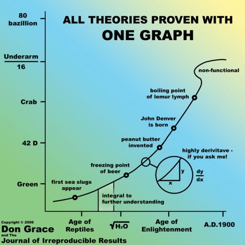
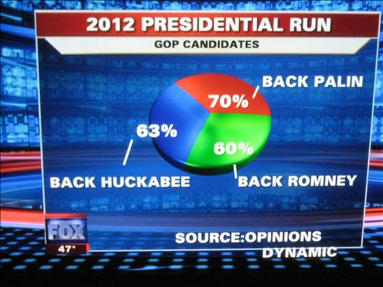
From JunkChartsNominated for Worst Graph of the Year, 2011

From Michael Friendly at York University

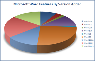
The 3-D pie chart is never a good idea.

Oops

I'm sure CNN and MSNBC have had some miserable graphs as well.

From Datavis

Maybe one of the best arguments against GUIs and "point-n-click" interfaces is that people produce crap like this.

There are a variety of tools available for making graphics, from the most basic to most elaborate, in R.

• Functions in base R

• Graphs menu in R Commander

• The lattice package (by Deepayan Sarkar, utilized in mosaic)

• The ggplot2 package (by Hadley Wickham, based on The Grammar of Graphics, for advanced users!)

  • A tutorial for ggplot2 I found on Rpubs.

• googleVis and other packages for advanced graphics, including 3-D and animation

The MASS package has a data set with nutritional content for 67 breakfast cereals. (If you are following along in R Commander, have to change shelf from numerical variable to a factor.)

require(MASS)
head(UScereal)

##                           mfr calories protein   fat sodium  fibre carbo
## 100% Bran                   N    212.1  12.121 3.030  393.9 30.303 15.15
## All-Bran                    K    212.1  12.121 3.030  787.9 27.273 21.21
## All-Bran with Extra Fiber   K    100.0   8.000 0.000  280.0 28.000 16.00
## Apple Cinnamon Cheerios     G    146.7   2.667 2.667  240.0  2.000 14.00
## Apple Jacks                 K    110.0   2.000 0.000  125.0  1.000 11.00
## Basic 4                     G    173.3   4.000 2.667  280.0  2.667 24.00
##                           sugars shelf potassium vitamins
## 100% Bran                  18.18     3    848.48 enriched
## All-Bran                   15.15     3    969.70 enriched
## All-Bran with Extra Fiber   0.00     3    660.00 enriched
## Apple Cinnamon Cheerios    13.33     1     93.33 enriched
## Apple Jacks                14.00     2     30.00 enriched
## Basic 4                    10.67     3    133.33 enriched

I have a hypothesis that cereals sold on the top shelf contain more fibre than cereals sold on the middle or bottom shelves.

Let's draw some graphs to compare this, using a variety of tools.

• EXCEL
• Base R
• lattice package
• ggplot2 package

yuck

I'm not sure I could reproduce the clicking I did to make this mediocre graph.

boxplot(fibre ~ shelf, data = UScereal, xlab = "Shelf", ylab = "Fibre (g)", 
    main = "Base R", col = "dodgerblue")

require(lattice)  #this will load `lattice`
bwplot(fibre ~ factor(shelf), data = UScereal, col = "hotpink", fill = "wheat", 
    main = "Lattice")

require(ggplot2)  #this will load `ggplot2`
qplot(factor(shelf), fibre, data = UScereal, geom = "boxplot") + ggtitle("ggplot2")

It's also pretty straightforward to do with R Commander. The code is shown because it is made available in the Output window.

require(Rcmdr)
Boxplot(fibre ~ shelf, data = UScereal, main = "R Commander")

Remember that big box of Crayolas you had as a kid with all those funky colors like periwinkle and burnt sienna? R has even more choices...

grep("red", colors(), value = TRUE)  #all shades of red

##  [1] "darkred"         "indianred"       "indianred1"     
##  [4] "indianred2"      "indianred3"      "indianred4"     
##  [7] "mediumvioletred" "orangered"       "orangered1"     
## [10] "orangered2"      "orangered3"      "orangered4"     
## [13] "palevioletred"   "palevioletred1"  "palevioletred2" 
## [16] "palevioletred3"  "palevioletred4"  "red"            
## [19] "red1"            "red2"            "red3"           
## [22] "red4"            "violetred"       "violetred1"     
## [25] "violetred2"      "violetred3"      "violetred4"

colors()  #all colors, 657

##   [1] "white"                "aliceblue"            "antiquewhite"        
##   [4] "antiquewhite1"        "antiquewhite2"        "antiquewhite3"       
##   [7] "antiquewhite4"        "aquamarine"           "aquamarine1"         
##  [10] "aquamarine2"          "aquamarine3"          "aquamarine4"         
##  [13] "azure"                "azure1"               "azure2"              
##  [16] "azure3"               "azure4"               "beige"               
##  [19] "bisque"               "bisque1"              "bisque2"             
##  [22] "bisque3"              "bisque4"              "black"               
##  [25] "blanchedalmond"       "blue"                 "blue1"               
##  [28] "blue2"                "blue3"                "blue4"               
##  [31] "blueviolet"           "brown"                "brown1"              
##  [34] "brown2"               "brown3"               "brown4"              
##  [37] "burlywood"            "burlywood1"           "burlywood2"          
##  [40] "burlywood3"           "burlywood4"           "cadetblue"           
##  [43] "cadetblue1"           "cadetblue2"           "cadetblue3"          
##  [46] "cadetblue4"           "chartreuse"           "chartreuse1"         
##  [49] "chartreuse2"          "chartreuse3"          "chartreuse4"         
##  [52] "chocolate"            "chocolate1"           "chocolate2"          
##  [55] "chocolate3"           "chocolate4"           "coral"               
##  [58] "coral1"               "coral2"               "coral3"              
##  [61] "coral4"               "cornflowerblue"       "cornsilk"            
##  [64] "cornsilk1"            "cornsilk2"            "cornsilk3"           
##  [67] "cornsilk4"            "cyan"                 "cyan1"               
##  [70] "cyan2"                "cyan3"                "cyan4"               
##  [73] "darkblue"             "darkcyan"             "darkgoldenrod"       
##  [76] "darkgoldenrod1"       "darkgoldenrod2"       "darkgoldenrod3"      
##  [79] "darkgoldenrod4"       "darkgray"             "darkgreen"           
##  [82] "darkgrey"             "darkkhaki"            "darkmagenta"         
##  [85] "darkolivegreen"       "darkolivegreen1"      "darkolivegreen2"     
##  [88] "darkolivegreen3"      "darkolivegreen4"      "darkorange"          
##  [91] "darkorange1"          "darkorange2"          "darkorange3"         
##  [94] "darkorange4"          "darkorchid"           "darkorchid1"         
##  [97] "darkorchid2"          "darkorchid3"          "darkorchid4"         
## [100] "darkred"              "darksalmon"           "darkseagreen"        
## [103] "darkseagreen1"        "darkseagreen2"        "darkseagreen3"       
## [106] "darkseagreen4"        "darkslateblue"        "darkslategray"       
## [109] "darkslategray1"       "darkslategray2"       "darkslategray3"      
## [112] "darkslategray4"       "darkslategrey"        "darkturquoise"       
## [115] "darkviolet"           "deeppink"             "deeppink1"           
## [118] "deeppink2"            "deeppink3"            "deeppink4"           
## [121] "deepskyblue"          "deepskyblue1"         "deepskyblue2"        
## [124] "deepskyblue3"         "deepskyblue4"         "dimgray"             
## [127] "dimgrey"              "dodgerblue"           "dodgerblue1"         
## [130] "dodgerblue2"          "dodgerblue3"          "dodgerblue4"         
## [133] "firebrick"            "firebrick1"           "firebrick2"          
## [136] "firebrick3"           "firebrick4"           "floralwhite"         
## [139] "forestgreen"          "gainsboro"            "ghostwhite"          
## [142] "gold"                 "gold1"                "gold2"               
## [145] "gold3"                "gold4"                "goldenrod"           
## [148] "goldenrod1"           "goldenrod2"           "goldenrod3"          
## [151] "goldenrod4"           "gray"                 "gray0"               
## [154] "gray1"                "gray2"                "gray3"               
## [157] "gray4"                "gray5"                "gray6"               
## [160] "gray7"                "gray8"                "gray9"               
## [163] "gray10"               "gray11"               "gray12"              
## [166] "gray13"               "gray14"               "gray15"              
## [169] "gray16"               "gray17"               "gray18"              
## [172] "gray19"               "gray20"               "gray21"              
## [175] "gray22"               "gray23"               "gray24"              
## [178] "gray25"               "gray26"               "gray27"              
## [181] "gray28"               "gray29"               "gray30"              
## [184] "gray31"               "gray32"               "gray33"              
## [187] "gray34"               "gray35"               "gray36"              
## [190] "gray37"               "gray38"               "gray39"              
## [193] "gray40"               "gray41"               "gray42"              
## [196] "gray43"               "gray44"               "gray45"              
## [199] "gray46"               "gray47"               "gray48"              
## [202] "gray49"               "gray50"               "gray51"              
## [205] "gray52"               "gray53"               "gray54"              
## [208] "gray55"               "gray56"               "gray57"              
## [211] "gray58"               "gray59"               "gray60"              
## [214] "gray61"               "gray62"               "gray63"              
## [217] "gray64"               "gray65"               "gray66"              
## [220] "gray67"               "gray68"               "gray69"              
## [223] "gray70"               "gray71"               "gray72"              
## [226] "gray73"               "gray74"               "gray75"              
## [229] "gray76"               "gray77"               "gray78"              
## [232] "gray79"               "gray80"               "gray81"              
## [235] "gray82"               "gray83"               "gray84"              
## [238] "gray85"               "gray86"               "gray87"              
## [241] "gray88"               "gray89"               "gray90"              
## [244] "gray91"               "gray92"               "gray93"              
## [247] "gray94"               "gray95"               "gray96"              
## [250] "gray97"               "gray98"               "gray99"              
## [253] "gray100"              "green"                "green1"              
## [256] "green2"               "green3"               "green4"              
## [259] "greenyellow"          "grey"                 "grey0"               
## [262] "grey1"                "grey2"                "grey3"               
## [265] "grey4"                "grey5"                "grey6"               
## [268] "grey7"                "grey8"                "grey9"               
## [271] "grey10"               "grey11"               "grey12"              
## [274] "grey13"               "grey14"               "grey15"              
## [277] "grey16"               "grey17"               "grey18"              
## [280] "grey19"               "grey20"               "grey21"              
## [283] "grey22"               "grey23"               "grey24"              
## [286] "grey25"               "grey26"               "grey27"              
## [289] "grey28"               "grey29"               "grey30"              
## [292] "grey31"               "grey32"               "grey33"              
## [295] "grey34"               "grey35"               "grey36"              
## [298] "grey37"               "grey38"               "grey39"              
## [301] "grey40"               "grey41"               "grey42"              
## [304] "grey43"               "grey44"               "grey45"              
## [307] "grey46"               "grey47"               "grey48"              
## [310] "grey49"               "grey50"               "grey51"              
## [313] "grey52"               "grey53"               "grey54"              
## [316] "grey55"               "grey56"               "grey57"              
## [319] "grey58"               "grey59"               "grey60"              
## [322] "grey61"               "grey62"               "grey63"              
## [325] "grey64"               "grey65"               "grey66"              
## [328] "grey67"               "grey68"               "grey69"              
## [331] "grey70"               "grey71"               "grey72"              
## [334] "grey73"               "grey74"               "grey75"              
## [337] "grey76"               "grey77"               "grey78"              
## [340] "grey79"               "grey80"               "grey81"              
## [343] "grey82"               "grey83"               "grey84"              
## [346] "grey85"               "grey86"               "grey87"              
## [349] "grey88"               "grey89"               "grey90"              
## [352] "grey91"               "grey92"               "grey93"              
## [355] "grey94"               "grey95"               "grey96"              
## [358] "grey97"               "grey98"               "grey99"              
## [361] "grey100"              "honeydew"             "honeydew1"           
## [364] "honeydew2"            "honeydew3"            "honeydew4"           
## [367] "hotpink"              "hotpink1"             "hotpink2"            
## [370] "hotpink3"             "hotpink4"             "indianred"           
## [373] "indianred1"           "indianred2"           "indianred3"          
## [376] "indianred4"           "ivory"                "ivory1"              
## [379] "ivory2"               "ivory3"               "ivory4"              
## [382] "khaki"                "khaki1"               "khaki2"              
## [385] "khaki3"               "khaki4"               "lavender"            
## [388] "lavenderblush"        "lavenderblush1"       "lavenderblush2"      
## [391] "lavenderblush3"       "lavenderblush4"       "lawngreen"           
## [394] "lemonchiffon"         "lemonchiffon1"        "lemonchiffon2"       
## [397] "lemonchiffon3"        "lemonchiffon4"        "lightblue"           
## [400] "lightblue1"           "lightblue2"           "lightblue3"          
## [403] "lightblue4"           "lightcoral"           "lightcyan"           
## [406] "lightcyan1"           "lightcyan2"           "lightcyan3"          
## [409] "lightcyan4"           "lightgoldenrod"       "lightgoldenrod1"     
## [412] "lightgoldenrod2"      "lightgoldenrod3"      "lightgoldenrod4"     
## [415] "lightgoldenrodyellow" "lightgray"            "lightgreen"          
## [418] "lightgrey"            "lightpink"            "lightpink1"          
## [421] "lightpink2"           "lightpink3"           "lightpink4"          
## [424] "lightsalmon"          "lightsalmon1"         "lightsalmon2"        
## [427] "lightsalmon3"         "lightsalmon4"         "lightseagreen"       
## [430] "lightskyblue"         "lightskyblue1"        "lightskyblue2"       
## [433] "lightskyblue3"        "lightskyblue4"        "lightslateblue"      
## [436] "lightslategray"       "lightslategrey"       "lightsteelblue"      
## [439] "lightsteelblue1"      "lightsteelblue2"      "lightsteelblue3"     
## [442] "lightsteelblue4"      "lightyellow"          "lightyellow1"        
## [445] "lightyellow2"         "lightyellow3"         "lightyellow4"        
## [448] "limegreen"            "linen"                "magenta"             
## [451] "magenta1"             "magenta2"             "magenta3"            
## [454] "magenta4"             "maroon"               "maroon1"             
## [457] "maroon2"              "maroon3"              "maroon4"             
## [460] "mediumaquamarine"     "mediumblue"           "mediumorchid"        
## [463] "mediumorchid1"        "mediumorchid2"        "mediumorchid3"       
## [466] "mediumorchid4"        "mediumpurple"         "mediumpurple1"       
## [469] "mediumpurple2"        "mediumpurple3"        "mediumpurple4"       
## [472] "mediumseagreen"       "mediumslateblue"      "mediumspringgreen"   
## [475] "mediumturquoise"      "mediumvioletred"      "midnightblue"        
## [478] "mintcream"            "mistyrose"            "mistyrose1"          
## [481] "mistyrose2"           "mistyrose3"           "mistyrose4"          
## [484] "moccasin"             "navajowhite"          "navajowhite1"        
## [487] "navajowhite2"         "navajowhite3"         "navajowhite4"        
## [490] "navy"                 "navyblue"             "oldlace"             
## [493] "olivedrab"            "olivedrab1"           "olivedrab2"          
## [496] "olivedrab3"           "olivedrab4"           "orange"              
## [499] "orange1"              "orange2"              "orange3"             
## [502] "orange4"              "orangered"            "orangered1"          
## [505] "orangered2"           "orangered3"           "orangered4"          
## [508] "orchid"               "orchid1"              "orchid2"             
## [511] "orchid3"              "orchid4"              "palegoldenrod"       
## [514] "palegreen"            "palegreen1"           "palegreen2"          
## [517] "palegreen3"           "palegreen4"           "paleturquoise"       
## [520] "paleturquoise1"       "paleturquoise2"       "paleturquoise3"      
## [523] "paleturquoise4"       "palevioletred"        "palevioletred1"      
## [526] "palevioletred2"       "palevioletred3"       "palevioletred4"      
## [529] "papayawhip"           "peachpuff"            "peachpuff1"          
## [532] "peachpuff2"           "peachpuff3"           "peachpuff4"          
## [535] "peru"                 "pink"                 "pink1"               
## [538] "pink2"                "pink3"                "pink4"               
## [541] "plum"                 "plum1"                "plum2"               
## [544] "plum3"                "plum4"                "powderblue"          
## [547] "purple"               "purple1"              "purple2"             
## [550] "purple3"              "purple4"              "red"                 
## [553] "red1"                 "red2"                 "red3"                
## [556] "red4"                 "rosybrown"            "rosybrown1"          
## [559] "rosybrown2"           "rosybrown3"           "rosybrown4"          
## [562] "royalblue"            "royalblue1"           "royalblue2"          
## [565] "royalblue3"           "royalblue4"           "saddlebrown"         
## [568] "salmon"               "salmon1"              "salmon2"             
## [571] "salmon3"              "salmon4"              "sandybrown"          
## [574] "seagreen"             "seagreen1"            "seagreen2"           
## [577] "seagreen3"            "seagreen4"            "seashell"            
## [580] "seashell1"            "seashell2"            "seashell3"           
## [583] "seashell4"            "sienna"               "sienna1"             
## [586] "sienna2"              "sienna3"              "sienna4"             
## [589] "skyblue"              "skyblue1"             "skyblue2"            
## [592] "skyblue3"             "skyblue4"             "slateblue"           
## [595] "slateblue1"           "slateblue2"           "slateblue3"          
## [598] "slateblue4"           "slategray"            "slategray1"          
## [601] "slategray2"           "slategray3"           "slategray4"          
## [604] "slategrey"            "snow"                 "snow1"               
## [607] "snow2"                "snow3"                "snow4"               
## [610] "springgreen"          "springgreen1"         "springgreen2"        
## [613] "springgreen3"         "springgreen4"         "steelblue"           
## [616] "steelblue1"           "steelblue2"           "steelblue3"          
## [619] "steelblue4"           "tan"                  "tan1"                
## [622] "tan2"                 "tan3"                 "tan4"                
## [625] "thistle"              "thistle1"             "thistle2"            
## [628] "thistle3"             "thistle4"             "tomato"              
## [631] "tomato1"              "tomato2"              "tomato3"             
## [634] "tomato4"              "turquoise"            "turquoise1"          
## [637] "turquoise2"           "turquoise3"           "turquoise4"          
## [640] "violet"               "violetred"            "violetred1"          
## [643] "violetred2"           "violetred3"           "violetred4"          
## [646] "wheat"                "wheat1"               "wheat2"              
## [649] "wheat3"               "wheat4"               "whitesmoke"          
## [652] "yellow"               "yellow1"              "yellow2"             
## [655] "yellow3"              "yellow4"              "yellowgreen"

Some of you don't like boxplots. You like plots of means with \(\pm 1\) standard error. That's reasonable. I think the easiest way is to utilize the plotMeans function in Rcmdr, or use the GUI.

require(Rcmdr)
plotMeans(UScereal$fibre, factor(UScereal$shelf), error.bars = "se")

Let's see a scatterplot of calories vs sugars, using four different packages.

plot(calories~sugars,data=UScereal)

require(lattice)
xyplot(calories~sugars,data=UScereal)

require(ggplot2)
ggplot(data=UScereal, aes(x=sugars, y=calories)) +
    geom_point(shape=1) +     # Use hollow circles
    geom_smooth(method=lm)    # Add linear regression line

require(Rcmdr)
scatterplot(calories~sugars,data=UScereal)

• To create your own R Markdown file, first go to File in RStudio and choose New File --> R Markdown.

• I made a R Markdown script that will:

  • Create boxplots of the fibre variable by shelf in the UScereal dataset.
  • Run an ANOVA to see if there are significant difference for fibre content based on the shelf
  • Write up an intelligent conclusion.

• When you are ready, you push the Knit HTML icon. This utilizes the knitr package to make your report.

• RPubs Information @ RPubs, brought to you by the folks at RStudio!

• Yihui Xie Yihui Xie is a graduate student at Iowa State who is quite good at graphics and R.

• Video Yihui made a video on getting started with R Markdown.

• Xie He's quite the young evangelist of reproducible research.

R Markdown

Some of our results for the "native" model (i.e. what variables predict whether a plant species in Kentucky is native or not)

I used this R Markdown .Rmd file with RStudio and knitr via the ball-of-yarn icon to produce this HTML file

Sweave (for advanced users!)

Charles Geyer A Sweave tutorial.

I used this Sweave .Rnw file ,combining LaTeX and R Code, and compiled it with RStudio to produce this .pdf file.

To make things easy, we'll use the built-in KidsFeet data set in the mosaic package. Is there a difference in width of foot between 4th grade boys vs girls?

require(mosaic)
KidsFeet

##        name birthmonth birthyear length width sex biggerfoot domhand
## 1     David          5        88   24.4   8.4   B          L       R
## 2      Lars         10        87   25.4   8.8   B          L       L
## 3      Zach         12        87   24.5   9.7   B          R       R
## 4      Josh          1        88   25.2   9.8   B          L       R
## 5      Lang          2        88   25.1   8.9   B          L       R
## 6    Scotty          3        88   25.7   9.7   B          R       R
## 7    Edward          2        88   26.1   9.6   B          L       R
## 8   Caitlin          6        88   23.0   8.8   G          L       R
## 9   Eleanor          5        88   23.6   9.3   G          R       R
## 10    Damon          9        88   22.9   8.8   B          R       L
## 11     Mark          9        87   27.5   9.8   B          R       R
## 12      Ray          3        88   24.8   8.9   B          L       R
## 13      Cal          8        87   26.1   9.1   B          L       R
## 14      Cam          3        88   27.0   9.8   B          L       R
## 15    Julie         11        87   26.0   9.3   G          L       R
## 16     Kate          4        88   23.7   7.9   G          R       R
## 17 Caroline         12        87   24.0   8.7   G          R       L
## 18   Maggie          3        88   24.7   8.8   G          R       R
## 19      Lee          6        88   26.7   9.0   G          L       L
## 20  Heather          3        88   25.5   9.5   G          R       R
## 21     Andy          6        88   24.0   9.2   B          R       R
## 22     Josh          7        88   24.4   8.6   B          L       R
## 23    Laura          9        88   24.0   8.3   G          R       L
## 24    Erica          9        88   24.5   9.0   G          L       R
## 25    Peggy         10        88   24.2   8.1   G          L       R
## 26     Glen          7        88   27.1   9.4   B          L       R
## 27     Abby          2        88   26.1   9.5   G          L       R
## 28    David         12        87   25.5   9.5   B          R       R
## 29     Mike         11        88   24.2   8.9   B          L       R
## 30   Dwayne          8        88   23.9   9.3   B          R       L
## 31 Danielle          6        88   24.0   9.3   G          L       R
## 32  Caitlin          7        88   22.5   8.6   G          R       R
## 33    Leigh          3        88   24.5   8.6   G          L       R
## 34    Dylan          4        88   23.6   9.0   B          R       L
## 35    Peter          4        88   24.7   8.6   B          R       L
## 36   Hannah          3        88   22.9   8.5   G          L       R
## 37 Teshanna          3        88   26.0   9.0   G          L       R
## 38   Hayley          1        88   21.6   7.9   G          R       R
## 39   Alisha          9        88   24.6   8.8   G          L       R

We need to...

• form a hypothesis

• collect data

• store data

• graph data so we can visualize what is there

• analyze data

• create a report to share our results

bwplot(y~x,data=dataset) (requires mosaic)

plotMeans(dataset$y,dataset$x) (requires Rcmdr)

favstats(y~x,data=dataset) (requires mosaic)

t.test(y~x,data=dataset)

Use help(function) to learn more about a function and its many options!

R Markdown: Start your file in RStudio by: File-->New File-->R Markdown. Click on the blue ? for help and the ball of yarn to knit your report!

If you think you have a good report, email me your .Rmd file. I should be able to reproduce your analyses.

You could also send me your .html file or you could publish it to Rpubs or to your own web page, blog, etc.

An example of someone else creating a reproducible report.

Jeromy Anglin's blog

His R Markdown script

One can make the Rosling-Gapminder style motion graphs in R. This requires the googleVis package.

Some info about including these graphs in presentations from Markus Gesmann.

RpubsSome help on googleVis.

require(googleVis)
demo(WorldBank)

If you type that into the R console, we can play with a demo of the Gapminder data in the web browser. How freaking cool is this???

An extensive database maintained by the Watershed Studies Institute dates back to 1988.

The variables I requested included:

• Elevation of Lake (feet)

• Temperature (celsius)

• Dissolved Oxygen (mg/L)

• pH

• Chlorophyll-a ( \(\mu\) g/L)

Code for KenLake data (you won't see the motion chart unless you have the data and run the code; I can't post this data--this graph isn't really ready for "prime-time" yet)

Eventually do this with the Mexican Cut salamanders???

Do you have data you'd like to see visualized with Motion Charts?