Geospatial data in R

21/06/2020

Useful resources

CRAN task view for spatial data:
https://cran.r-project.org/web/views/Spatial.html

Geocomputation with R:
https://geocompr.robinlovelace.net

sf package cheatsheet:
https://github.com/rstudio/cheatsheets/blob/master/sf.pdf

sf package overview:
https://r-spatial.github.io/sf/articles/sf1.html

Geospatial data

Generally refers to spatial data that is positioned on Earth

1D: a point on a line
2D: a point on an x-y plane
3D: x & y & z (altitude)
4D: x & y & z & time

Sources of geospatial data

GPS points (e.g., collected on your phone)
Country/state/property boundaries (e.g., from gov agency)
Georeferenced images (e.g., sat imagery, drone photos)

Coordinate Reference Systems (CRSes)

CRSes and projections and datums
- a CRS consists of a geometric model/ellipsoid of the shape of the earth and a datum (origin of the coordinates, and their units)
CRS can be geographic or projected
- Geo - points on an ellipsoid, in degrees
- Proj - points on a plane, in metres
If the earth were a perfect sphere, we could have a global CRS
- But it’s not. So we don’t.

Geographic

Most common; global format (WGS84)
Example: -19.327459˚, 146.760092˚
- lat, long = y, x
- x, y = long, lat
Degrees of latitude: north-south
Degrees of longitude: east-west
Note:
- Be careful when longitudes cross the prime meridian
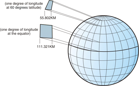
- 1 degree of latitude = 111km anywhere on the globe
- 1 degree of longitude varies depending on latitude

Geographic - latitude

IBM - Geographic coordinate system

Geographic - longitude

Geographic - varying distances

Projected

A flat representation of the spherical planet
- Like any printed map
Example: 1585278 East, -2497674 North
Units in, e.g., metres
Convenient to work with
- Areas and distances are all in metres (or square metres)

Two main formats - raster

Raster = matrix or grid
- one file can have multiple bands
  - Most commonly encountered in sat imagery: Red & Green & Blue bands
- GeoTiff - georeferenced TIFF image
- Can be geographic or projected
  - Geographic: map units will be in degrees
  - Projected: map units will be, e.g., metres

Two main formats - vector

Vector = points that may or may not be connected
- Shapefile
- Delimited text with X & Y columns
- Simple Features - standard for geospatial data exchange - https://en.wikipedia.org/wiki/Simple_Features

GIS tools

ArcGIS (powerful, expensive, frustrating)
QGIS (free & open source, still frustrating)
- Great for rapid visualisations
GDAL
- used behind-the-scenes in many other software
- Can also be used on the command line
PostgreSQL with PostGIS extension
- Probably overkill for most research projects
- Great for long-term storage and analysis
Google Earth Engine
- Very powerful way of dealing with rasters, esp. sat imagery

GIS in R

Packages:
- raster
- sp: SPatial
  - older, being used less
- sf: Simple Features
  - use this for any new code you write
  - objects are data frames, and thus integrate with tidyverse; also, it actually works

sf package

Objects are dataframes
- Standard dataframe, with a geometry column added that contains the geometry info for each row
Example functions
- st_read() to read in spatial data in various formats
- st_intersection to calculate spatial overlaps
- st_transform to transform between CRSes (e.g., geographic to projected)
- st_distance to calculate distance in the correct units
- st_area to calculate area in the correct units
The st prefix stands for spatio-temporal

Reading CSV text files

townFile <- 'https://raw.githubusercontent.com/stewartmacdonald/species-mapping-in-r/master/towns.csv'
townDF <- read.csv(townFile) %>%
  
  # select the long and lat cols from the data frame
  st_as_sf(coords = c("long", "lat"),
               crs=4326,
               remove=FALSE) %>%
    
    # transform from geographical to projected (Aus Albers Equal Area)
    st_transform(3577)

townDF

townDF

## Simple feature collection with 16 features and 3 fields
## geometry type:  POINT
## dimension:      XY
## bbox:           xmin: -1565304 ymin: -4192601 xmax: 2043345 ymax: -1314021
## CRS:            EPSG:3577
## First 10 features:
##           name       lat     long                   geometry
## 1   Meekathara -26.57581 118.4910  POINT (-1326990 -2949464)
## 2       Cairns -16.92856 145.7645   POINT (1467641 -1882911)
## 3   Kalgoorlie -30.75226 121.4708 POINT (-996488.6 -3388716)
## 4     Karratha -20.73579 116.8447  POINT (-1565304 -2318944)
## 5       Broome -17.95775 122.2235  POINT (-1034732 -1957122)
## 6  Coober Pedy -29.01390 134.7535  POINT (265066.6 -3155598)
## 7  Charleville -26.42671 146.2763   POINT (1403929 -2941042)
## 8       Mt Isa -20.72166 139.4893  POINT (774989.2 -2247140)
## 9    Kununurra -15.78214 128.7375 POINT (-351728.4 -1681972)
## 10      Darwin -12.45277 130.8393 POINT (-128455.3 -1314021)

Plotting points

plot(townDF$long, townDF$lat)

Reading in GeoJSON (or similar)

worldFile <- 'https://github.com/stewartmacdonald/covid-19/raw/master/world.geojson'
ausShp <- st_read(worldFile, quiet=TRUE) %>%
  dplyr::filter(ADMIN == 'Australia')

ausShp

## Simple feature collection with 1 feature and 94 fields
## geometry type:  MULTIPOLYGON
## dimension:      XY
## bbox:           xmin: 112.9082 ymin: -54.74922 xmax: 158.9589 ymax: -10.05176
## CRS:            4326
##        featurecla scalerank LABELRANK SOVEREIGNT SOV_A3 ADM0_DIF LEVEL    TYPE
## 1 Admin-0 country         1         2  Australia    AU1        1     2 Country
##       ADMIN ADM0_A3 GEOU_DIF   GEOUNIT GU_A3 SU_DIF   SUBUNIT SU_A3 BRK_DIFF
## 1 Australia     AUS        0 Australia   AUS      0 Australia   AUS        0
##        NAME NAME_LONG BRK_A3  BRK_NAME BRK_GROUP ABBREV POSTAL
## 1 Australia Australia    AUS Australia      <NA>   Auz.     AU
##                   FORMAL_EN FORMAL_FR NAME_CIAWF NOTE_ADM0 NOTE_BRK NAME_SORT
## 1 Commonwealth of Australia      <NA>  Australia      <NA>     <NA> Australia
##   NAME_ALT MAPCOLOR7 MAPCOLOR8 MAPCOLOR9 MAPCOLOR13  POP_EST POP_RANK
## 1     <NA>         1         2         2          7 23232413       15
##   GDP_MD_EST POP_YEAR LASTCENSUS GDP_YEAR                    ECONOMY
## 1    1189000     2017       2006     2016 2. Developed region: nonG7
##             INCOME_GRP WIKIPEDIA FIPS_10_ ISO_A2 ISO_A3 ISO_A3_EH ISO_N3 UN_A3
## 1 1. High income: OECD       -99       AS     AU    AUS       AUS    036   036
##   WB_A2 WB_A3 WOE_ID WOE_ID_EH
## 1    AU   AUS    -90  23424748
##                                                                            WOE_NOTE
## 1 Includes Ashmore and Cartier Islands (23424749) and Coral Sea Islands (23424790).
##   ADM0_A3_IS ADM0_A3_US ADM0_A3_UN ADM0_A3_WB CONTINENT REGION_UN
## 1        AUS        AUS        -99        -99   Oceania   Oceania
##                   SUBREGION           REGION_WB NAME_LEN LONG_LEN ABBREV_LEN
## 1 Australia and New Zealand East Asia & Pacific        9        9          4
##   TINY HOMEPART MIN_ZOOM MIN_LABEL MAX_LABEL      NE_ID WIKIDATAID  NAME_AR
## 1  -99        1        0       1.7       5.7 1159320355       Q408 أستراليا
##     NAME_BN    NAME_DE   NAME_EN   NAME_ES   NAME_FR   NAME_EL  NAME_HI
## 1 অস্ট্রেলিয়া Australien Australia Australia Australie Αυστραλία ऑस्ट्रेलिया
##      NAME_HU   NAME_ID   NAME_IT        NAME_JA        NAME_KO   NAME_NL
## 1 Ausztrália Australia Australia オーストラリア 오스트레일리아 Australië
##     NAME_PL   NAME_PT   NAME_RU    NAME_SV    NAME_TR NAME_VI  NAME_ZH
## 1 Australia Austrália Австралия Australien Avustralya      Úc 澳大利亚
##                         geometry
## 1 MULTIPOLYGON (((143.1789 -1...

Plotting lines

plot(ausShp, col='white', max.plot=1, reset=FALSE)
points(townDF$long, townDF$lat, pch=16, col='lightgrey')
plot(st_transform(townDF, 4326), pch=16, col='black', add=T)

## Warning in plot.sf(st_transform(townDF, 4326), pch = 16, col = "black", :
## ignoring all but the first attribute

Plotting with ggplot

ggplot() +
  geom_sf(data=ausShp)

Plotting with ggplot

ggplot() +
  geom_sf(data=ausShp) + 
  geom_sf(data=townDF)

Styling

ggplot() +
  geom_sf(data=ausShp) + 
  geom_sf(data=townDF, aes(colour=name)) +
  theme_classic()

Styling

ggplot() +
  geom_sf(data=ausShp) + geom_sf(data=townDF, aes(colour=name)) +
  theme_classic() + ylim(-45, -10)

Styling

ggplot() +
  geom_sf(data=ausShp) + geom_sf(data=townDF, aes(colour=name)) +
  theme_classic() + ylim(-45, -10) +
  coord_sf(datum = NA) # to remove graticules and axes

A better Australia

ausFile <- 'https://raw.githubusercontent.com/stewartmacdonald/species-mapping-in-r/master/australia.geojson'
ausShp <- st_read(ausFile, quiet=TRUE)
ausShp

## Simple feature collection with 8 features and 12 fields
## geometry type:  MULTIPOLYGON
## dimension:      XY
## bbox:           xmin: 112.9072 ymin: -43.64806 xmax: 159.1019 ymax: -10.05139
## CRS:            4283
##   FIPS_ADMIN GMI_ADMIN                   ADMIN_NAME FIPS_CNTRY CNTRY_NAME
## 1       AS03   AUS-NTR           Northern Territory         AS  Australia
## 2       AS04   AUS-QNS                   Queensland         AS  Australia
## 3       AS01   AUS-ACT Australian Capital Territory         AS  Australia
## 4       AS02   AUS-NSW              New South Wales         AS  Australia
## 5       AS07   AUS-VCT                     Victoria         AS  Australia
## 6       AS08   AUS-WAS            Western Australia         AS  Australia
## 7       AS05   AUS-SAS              South Australia         AS  Australia
## 8       AS06   AUS-TSM                     Tasmania         AS  Australia
##                  REGION CONTINENT POP_ADMIN  SQKM_ADMIN SQMI_ADMIN  TYPE_ENG
## 1 Australia/New Zealand Australia    161294 1352365.000  522148.09 Territory
## 2 Australia/New Zealand Australia   3107362 1733475.000  669294.69     State
## 3 Australia/New Zealand Australia    292475    2342.295     904.36 Territory
## 4 Australia/New Zealand Australia   6338919  803110.812  310081.09     State
## 5 Australia/New Zealand Australia   4354611  227781.406   87946.40     State
## 6 Australia/New Zealand Australia   1655588 2533628.000  978233.81     State
## 7 Australia/New Zealand Australia   1445153  985308.500  380427.59     State
## 8 Australia/New Zealand Australia    472122   68131.477   26305.56     State
##    TYPE_LOC                       geometry
## 1 Territory MULTIPOLYGON (((136.6622 -1...
## 2     State MULTIPOLYGON (((146.8208 -1...
## 3 Territory MULTIPOLYGON (((149.0428 -3...
## 4     State MULTIPOLYGON (((141.0027 -2...
## 5     State MULTIPOLYGON (((145.3558 -3...
## 6     State MULTIPOLYGON (((113.0617 -2...
## 7     State MULTIPOLYGON (((133.565 -32...
## 8     State MULTIPOLYGON (((144.8889 -4...

Plotting

ggplot() +
  geom_sf(data=ausShp) +
  theme_classic() + coord_sf(datum = NA)

Plotting

ggplot() +
  geom_sf(data=ausShp) + geom_sf(data=townDF) +
  theme_classic() + coord_sf(datum = NA)

Plotting

ggplot() +
  geom_sf(data=ausShp, aes(fill=ADMIN_NAME)) + geom_sf(data=townDF) +
  theme_classic() + coord_sf(datum = NA)

Spatial operations

What state is each town in?

townDF

## Simple feature collection with 16 features and 3 fields
## geometry type:  POINT
## dimension:      XY
## bbox:           xmin: -1565304 ymin: -4192601 xmax: 2043345 ymax: -1314021
## CRS:            EPSG:3577
## First 10 features:
##           name       lat     long                   geometry
## 1   Meekathara -26.57581 118.4910  POINT (-1326990 -2949464)
## 2       Cairns -16.92856 145.7645   POINT (1467641 -1882911)
## 3   Kalgoorlie -30.75226 121.4708 POINT (-996488.6 -3388716)
## 4     Karratha -20.73579 116.8447  POINT (-1565304 -2318944)
## 5       Broome -17.95775 122.2235  POINT (-1034732 -1957122)
## 6  Coober Pedy -29.01390 134.7535  POINT (265066.6 -3155598)
## 7  Charleville -26.42671 146.2763   POINT (1403929 -2941042)
## 8       Mt Isa -20.72166 139.4893  POINT (774989.2 -2247140)
## 9    Kununurra -15.78214 128.7375 POINT (-351728.4 -1681972)
## 10      Darwin -12.45277 130.8393 POINT (-128455.3 -1314021)

Spatial operations

Append the states’ attributes to the towns they contain

town2DF <- st_join(townDF, st_transform(ausShp, 3577))
town2DF

## Simple feature collection with 16 features and 15 fields
## geometry type:  POINT
## dimension:      XY
## bbox:           xmin: -1565304 ymin: -4192601 xmax: 2043345 ymax: -1314021
## CRS:            EPSG:3577
## First 10 features:
##           name       lat     long FIPS_ADMIN GMI_ADMIN         ADMIN_NAME
## 1   Meekathara -26.57581 118.4910       AS08   AUS-WAS  Western Australia
## 2       Cairns -16.92856 145.7645       AS04   AUS-QNS         Queensland
## 3   Kalgoorlie -30.75226 121.4708       AS08   AUS-WAS  Western Australia
## 4     Karratha -20.73579 116.8447       AS08   AUS-WAS  Western Australia
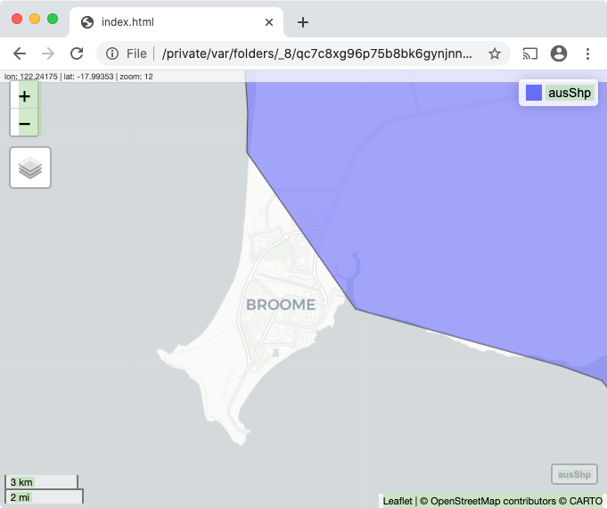
## 5       Broome -17.95775 122.2235       <NA>      <NA>               <NA>
## 6  Coober Pedy -29.01390 134.7535       AS05   AUS-SAS    South Australia
## 7  Charleville -26.42671 146.2763       AS04   AUS-QNS         Queensland
## 8       Mt Isa -20.72166 139.4893       AS04   AUS-QNS         Queensland
## 9    Kununurra -15.78214 128.7375       AS08   AUS-WAS  Western Australia
## 10      Darwin -12.45277 130.8393       AS03   AUS-NTR Northern Territory
##    FIPS_CNTRY CNTRY_NAME                REGION CONTINENT POP_ADMIN SQKM_ADMIN
## 1          AS  Australia Australia/New Zealand Australia   1655588  2533628.0
## 2          AS  Australia Australia/New Zealand Australia   3107362  1733475.0
## 3          AS  Australia Australia/New Zealand Australia   1655588  2533628.0
## 4          AS  Australia Australia/New Zealand Australia   1655588  2533628.0
## 5        <NA>       <NA>                  <NA>      <NA>        NA         NA
## 6          AS  Australia Australia/New Zealand Australia   1445153   985308.5
## 7          AS  Australia Australia/New Zealand Australia   3107362  1733475.0
## 8          AS  Australia Australia/New Zealand Australia   3107362  1733475.0
## 9          AS  Australia Australia/New Zealand Australia   1655588  2533628.0
## 10         AS  Australia Australia/New Zealand Australia    161294  1352365.0
##    SQMI_ADMIN  TYPE_ENG  TYPE_LOC                   geometry
## 1    978233.8     State     State  POINT (-1326990 -2949464)
## 2    669294.7     State     State   POINT (1467641 -1882911)
## 3    978233.8     State     State POINT (-996488.6 -3388716)
## 4    978233.8     State     State  POINT (-1565304 -2318944)
## 5          NA      <NA>      <NA>  POINT (-1034732 -1957122)
## 6    380427.6     State     State  POINT (265066.6 -3155598)
## 7    669294.7     State     State   POINT (1403929 -2941042)
## 8    669294.7     State     State  POINT (774989.2 -2247140)
## 9    978233.8     State     State POINT (-351728.4 -1681972)
## 10   522148.1 Territory Territory POINT (-128455.3 -1314021)

mapview - interactive spatial data

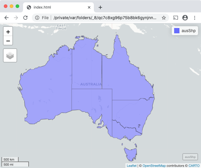
mapview::mapview(ausShp)

mapview - interactive spatial data

mapview::mapview(ausShp)

Plotting

ggplot() +
  geom_sf(data=ausShp, fill='white') +
  geom_sf(data=town2DF, aes(colour=ADMIN_NAME)) +
  theme_classic() + coord_sf(datum = NA)

Other operations

# Colours
red    <- '#f90000'
blue   <- '#0035f9'
purple <- '#8900f9'

# Mainland
aPts <- c(1,1, 2,2, 3,1, 4,1, 5,3, 4,5.5, 3.5,4,
          3,5, 2,5, 2,4, 1,5, 0,3, 1,1)
aPts <- matrix(aPts, ncol=2, byrow=T)
a <- st_polygon(list(aPts))

# Species range
bPts <- c(0,3, 5,3, 5,6, 0,6, 0,3)
bPts <- matrix(bPts, ncol=2, byrow=T)
b <- st_polygon(list(bPts))

Other operations

Convert to sf objects

mainland <- st_sf(data.frame(name='mainland', geom=st_sfc(a)),
                  agr='constant')

species <- st_sf(data.frame(name='species_range', geom=st_sfc(b)),
                 agr='constant')

both <- rbind(mainland, species)

Other operations

Plot mainland

ggplot() +
    geom_sf(data=mainland, fill=red,  alpha=0.5)

Other operations

Add species range

ggplot() +
    geom_sf(data=mainland, fill=red,  alpha=0.5) +
    geom_sf(data=species,  fill=blue, alpha=0.5)

Intersection

# returns the overlap between a and b. Order doesn't matter.
intersection <- st_intersection(mainland, species)
ggplot() +
  geom_sf(data=both, fill=NA) +
  geom_sf(data=intersection, fill=purple, alpha=0.5)

Difference

# returns the parts of 'b' that are outside of 'a'
differenceAB <- st_difference(species, mainland)
ggplot() +
  geom_sf(data=both, fill=NA) +
  geom_sf(data=differenceAB, fill=blue, alpha=0.5)

Difference - order matters

# returns the parts of 'b' that are outside of 'a'
differenceBA <- st_difference(mainland, species)
ggplot() +
  geom_sf(data=both, fill=NA) +
  geom_sf(data=differenceBA, fill=red, alpha=0.5)

Difference with buffer

# returns the parts of 'b' that are outside of 'a', with a small buffer
differenceAB <- st_difference(species, mainland)
differenceAB <- st_buffer(differenceAB, dist=0.1)
ggplot() +
  geom_sf(data=both, fill=NA) +
  geom_sf(data=differenceAB, fill=blue, alpha=0.5)

Union

# Merges two polygons into one
union <- st_union(species, mainland)
ggplot() +
  geom_sf(data=union, fill=purple, alpha=0.5)

Centroid

# Range centre
centre <- st_centroid(species)
ggplot() +
  geom_sf(data=species, fill=NA) +
  geom_sf(data=mainland, fill=red, alpha=0.5) +
  geom_sf(data=centre)

Within et al.

Is the centre of the species polygon within the mainland polygon?

v <- st_within(centre, mainland, sparse=F)      # true
v <- st_intersects(centre, mainland, sparse=F)  # true
v <- st_disjoint(centre, mainland, sparse=F)    # false

# Order matters
v <- st_contains(centre, mainland, sparse=F)    # false
v <- st_contains(mainland, centre, sparse=F)    # true

More info

species and mainland examples of spatial operations taken from:
https://github.com/stewartmacdonald/species-mapping-in-r

Base maps

#devtools::install_github('Chrisjb/basemapR')
library(basemapR)

townDF <- st_transform(townDF, 4326)

# create bbox from our sf object and expand it by 1km
bbox <- expand_bbox(st_bbox(townDF), X = 1000, Y = 1000)

ggplot() +
  base_map(st_bbox(townDF), increase_zoom=2, basemap='google-terrain') +
  geom_sf(data=townDF) +
  
  coord_sf(datum = NA,
           xlim = c(bbox['xmin'], bbox['xmax']),
           ylim = c(bbox['ymin'], bbox['ymax'])) +
  theme_minimal() +
  labs(caption = 'Map data \uA9 2020 Google')

## please cite: map data © 2020 Google

Base maps

## please cite: map data © 2020 Google

Base maps

## please cite: map data © 2020 Google