R basics
Farid FLICI
18-05-2020
Algerian R Users Group

Plan
- Data manipulation
- Data visualization
- Editing (R markdown)
Plan
Data manipulation
- Data Structures: vector of characters, matrix, datafram
- c(), re(), seq(), matrix(), data.frame()
- t(), melt(), merge()
- for (), if(), ifelse()
Data visualization
- plot(), lines(), points
- barplot()
Editing (R markdown)
- Installing R markdown,
- writing text,
- Equations, figures, tables
Data structures
a vector
c(1, 3, 4, 5, 6)
[1] 1 3 4 5 6
a sequence
seq(1, 9, by=1)
[1] 1 2 3 4 5 6 7 8 9
seq(1, 9, by=1)+3
[1] 4 5 6 7 8 9 10 11 12
Data structures
a repitition
rep(5, 6)
[1] 5 5 5 5 5 5
rep(NA, 6)
[1] NA NA NA NA NA NA
Data structures
a matrix
M <- matrix(c(1:20), byrow=T, ncol=5)
M
     [,1] [,2] [,3] [,4] [,5]
[1,]    1    2    3    4    5
[2,]    6    7    8    9   10
[3,]   11   12   13   14   15
[4,]   16   17   18   19   20
N <- matrix(c(1:20), byrow=F, ncol=5)
N
     [,1] [,2] [,3] [,4] [,5]
[1,]    1    5    9   13   17
[2,]    2    6   10   14   18
[3,]    3    7   11   15   19
[4,]    4    8   12   16   20
Data structures
a vector
M1 <- matrix(seq(18,20), ncol=1)
M1
     [,1]
[1,]   18
[2,]   19
[3,]   20
N1 <- matrix(seq(16,18), nrow=1)
N1
     [,1] [,2] [,3]
[1,]   16   17   18
Data structures
vectors
M2 <- M1+1
M2
     [,1]
[1,]   19
[2,]   20
[3,]   21
N2 <- N1*3
N2
     [,1] [,2] [,3]
[1,]   48   51   54
Data structures
M1
     [,1]
[1,]   18
[2,]   19
[3,]   20
N1
     [,1] [,2] [,3]
[1,]   16   17   18
M1%*%N1
     [,1] [,2] [,3]
[1,]  288  306  324
[2,]  304  323  342
[3,]  320  340  360
N1%*%M1
     [,1]
[1,]  971
Data structures
Matrices subsetting
M
     [,1] [,2] [,3] [,4] [,5]
[1,]    1    2    3    4    5
[2,]    6    7    8    9   10
[3,]   11   12   13   14   15
[4,]   16   17   18   19   20
M[, -1]
     [,1] [,2] [,3] [,4]
[1,]    2    3    4    5
[2,]    7    8    9   10
[3,]   12   13   14   15
[4,]   17   18   19   20
Data structures
Matrices subsetting
M
     [,1] [,2] [,3] [,4] [,5]
[1,]    1    2    3    4    5
[2,]    6    7    8    9   10
[3,]   11   12   13   14   15
[4,]   16   17   18   19   20
M[, c(-1,-2)]
     [,1] [,2] [,3]
[1,]    3    4    5
[2,]    8    9   10
[3,]   13   14   15
[4,]   18   19   20
M[-2,]
     [,1] [,2] [,3] [,4] [,5]
[1,]    1    2    3    4    5
[2,]   11   12   13   14   15
[3,]   16   17   18   19   20
Data structures
Matrices subsetting
M
     [,1] [,2] [,3] [,4] [,5]
[1,]    1    2    3    4    5
[2,]    6    7    8    9   10
[3,]   11   12   13   14   15
[4,]   16   17   18   19   20
subset(M, select=c(1:3))
     [,1] [,2] [,3]
[1,]    1    2    3
[2,]    6    7    8
[3,]   11   12   13
[4,]   16   17   18
M[3:4, 3:5]
     [,1] [,2] [,3]
[1,]   13   14   15
[2,]   18   19   20
Useful R functions
rbind(), cbind()
add some columns
M
     [,1] [,2] [,3] [,4] [,5]
[1,]    1    2    3    4    5
[2,]    6    7    8    9   10
[3,]   11   12   13   14   15
[4,]   16   17   18   19   20
M4 <- cbind(M, rep(1, nrow(M)))
M4
     [,1] [,2] [,3] [,4] [,5] [,6]
[1,]    1    2    3    4    5    1
[2,]    6    7    8    9   10    1
[3,]   11   12   13   14   15    1
[4,]   16   17   18   19   20    1
Useful R functions
rbind(), cbind()
add some columns
M
     [,1] [,2] [,3] [,4] [,5]
[1,]    1    2    3    4    5
[2,]    6    7    8    9   10
[3,]   11   12   13   14   15
[4,]   16   17   18   19   20
M5 <- cbind(M, matrix(rep(1), ncol=2, nrow=nrow(M)))
M5
     [,1] [,2] [,3] [,4] [,5] [,6] [,7]
[1,]    1    2    3    4    5    1    1
[2,]    6    7    8    9   10    1    1
[3,]   11   12   13   14   15    1    1
[4,]   16   17   18   19   20    1    1
Useful R functions
rbind(), cbind()
add some rows
M
     [,1] [,2] [,3] [,4] [,5]
[1,]    1    2    3    4    5
[2,]    6    7    8    9   10
[3,]   11   12   13   14   15
[4,]   16   17   18   19   20
M6 <- rbind(M, rep(1, ncol(M)))
M6
     [,1] [,2] [,3] [,4] [,5]
[1,]    1    2    3    4    5
[2,]    6    7    8    9   10
[3,]   11   12   13   14   15
[4,]   16   17   18   19   20
[5,]    1    1    1    1    1
Useful R functions
rbind(), cbind()
add some rows
M
     [,1] [,2] [,3] [,4] [,5]
[1,]    1    2    3    4    5
[2,]    6    7    8    9   10
[3,]   11   12   13   14   15
[4,]   16   17   18   19   20
M7 <- rbind(M, matrix(rep(1), nrow=2, ncol=ncol(M)))
M7
     [,1] [,2] [,3] [,4] [,5]
[1,]    1    2    3    4    5
[2,]    6    7    8    9   10
[3,]   11   12   13   14   15
[4,]   16   17   18   19   20
[5,]    1    1    1    1    1
[6,]    1    1    1    1    1
Useful R functions
subsetting
Example: form “M”, select only the “rows” having a value “>=” to “10” within columns “5”.
M
     [,1] [,2] [,3] [,4] [,5]
[1,]    1    2    3    4    5
[2,]    6    7    8    9   10
[3,]   11   12   13   14   15
[4,]   16   17   18   19   20
M[ M[ , 5]>=10, ]
     [,1] [,2] [,3] [,4] [,5]
[1,]    6    7    8    9   10
[2,]   11   12   13   14   15
[3,]   16   17   18   19   20
Useful R functions
subsetting
Select only columns 3,
M[ M[ , 5]>=10, 3]
[1] 8 13 18
length(M[ M[ , 5]>=10, 3])
[1] 3
Useful R functions
for() and if()
in M, we replace the values M[ ,2] <=10 by 10.
Ma <- M
Ma[ Ma[ ,2]<=10,2]<-rep(10,length(Ma[Ma[,2]<=10,2]))
Ma
     [,1] [,2] [,3] [,4] [,5]
[1,]    1   10    3    4    5
[2,]    6   10    8    9   10
[3,]   11   12   13   14   15
[4,]   16   17   18   19   20
or
Mb<-M
for (i in 1: nrow(Mb)){ if(Mb[i,2]<=10){Mb[i, 2]<-10}   }
Mb
     [,1] [,2] [,3] [,4] [,5]
[1,]    1   10    3    4    5
[2,]    6   10    8    9   10
[3,]   11   12   13   14   15
[4,]   16   17   18   19   20
Useful R functions
melt() and cast()
for example, we have a matrix \( tax \), indicating tax amount (in cells) for car by power (column) and year (rows)
tax<- matrix(seq(1000, 15000, by=1000 ), byrow = T, ncol=5)
colnames(tax)<-seq(2011, 2015)
rownames(tax)<-c(4,5,7)
tax
   2011  2012  2013  2014  2015
4  1000  2000  3000  4000  5000
5  6000  7000  8000  9000 10000
7 11000 12000 13000 14000 15000
Useful R functions
melt()
melt() allows to rewrite the matrix into 3 columns dataframe (power, year, tax)
library(reshape2)
tax2<-melt(tax)
colnames(tax2)<-c("power", "year", "tax")
tax2
   power year   tax
1      4 2011  1000
2      5 2011  6000
3      7 2011 11000
4      4 2012  2000
5      5 2012  7000
6      7 2012 12000
7      4 2013  3000
8      5 2013  8000
9      7 2013 13000
10     4 2014  4000
11     5 2014  9000
12     7 2014 14000
13     4 2015  5000
14     5 2015 10000
15     7 2015 15000
Useful R functions
cast()
cast() allows aggregating data, it is the adverse function for melt()
library(reshape2)
head(tax2)
  power year   tax
1     4 2011  1000
2     5 2011  6000
3     7 2011 11000
4     4 2012  2000
5     5 2012  7000
6     7 2012 12000
dcast(tax2, power~year, mean)
  power  2011  2012  2013  2014  2015
1     4  1000  2000  3000  4000  5000
2     5  6000  7000  8000  9000 10000
3     7 11000 12000 13000 14000 15000
We replace “mean” by “length” if we want to have counts on “cells”
Useful R functions
Examples
We create two dataframes
A <- data.frame(ID=seq(1,10), Age=c(15, 24, 32, 18, 46, 35, 38, 34, 46, 42), sex=c(1, 2, 2, 1, 1, 1, 2, 2, 1, 2), chl=c(0, 1, 2, 0, 3, 1, 2, 3, 2, 0))

B<- data.frame(ID=seq(6,15), wrk=c(1, 1, 0, 1,1, 0, 0, 1, 1, 0), std=c(1,1,2,2,3,3,4,4, 3, 2))

A
   ID Age sex chl
1   1  15   1   0
2   2  24   2   1
3   3  32   2   2
4   4  18   1   0
5   5  46   1   3
6   6  35   1   1
7   7  38   2   2
8   8  34   2   3
9   9  46   1   2
10 10  42   2   0
Examples
A <- data.frame(ID=seq(1,10), Age=c(15, 24, 32, 18, 46, 35, 38, 34, 46, 42), sex=c(1, 2, 2, 1, 1, 1, 2, 2, 1, 2), chl=c(0, 1, 2, 0, 3, 1, 2, 3, 2, 0))

B<- data.frame(ID=seq(6,15), wrk=c(1, 1, 0, 1,1, 0, 0, 1, 1, 0), std=c(1,1,2,2,3,3,4,4, 3, 2))

cbind.data.frame(A,"---"=rep("---"), B)
   ID Age sex chl --- ID wrk std
1   1  15   1   0 ---  6   1   1
2   2  24   2   1 ---  7   1   1
3   3  32   2   2 ---  8   0   2
4   4  18   1   0 ---  9   1   2
5   5  46   1   3 --- 10   1   3
6   6  35   1   1 --- 11   0   3
7   7  38   2   2 --- 12   0   4
8   8  34   2   3 --- 13   1   4
9   9  46   1   2 --- 14   1   3
10 10  42   2   0 --- 15   0   2
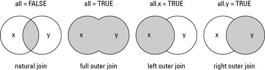
Different ways to merge A and B
Inner Join
C<-merge(x=A, y=B, by="ID", all=FALSE)
C
  ID Age sex chl wrk std
1  6  35   1   1   1   1
2  7  38   2   2   1   1
3  8  34   2   3   0   2
4  9  46   1   2   1   2
5 10  42   2   0   1   3
Different ways to merge A and B
left Join
D<-merge(x=A, y=B, by="ID", all.x=TRUE)
D
   ID Age sex chl wrk std
1   1  15   1   0  NA  NA
2   2  24   2   1  NA  NA
3   3  32   2   2  NA  NA
4   4  18   1   0  NA  NA
5   5  46   1   3  NA  NA
6   6  35   1   1   1   1
7   7  38   2   2   1   1
8   8  34   2   3   0   2
9   9  46   1   2   1   2
10 10  42   2   0   1   3
Different ways to merge A and B
Right Join
E<-merge(x=A, y=B, by="ID", all.y=TRUE)
E
   ID Age sex chl wrk std
1   6  35   1   1   1   1
2   7  38   2   2   1   1
3   8  34   2   3   0   2
4   9  46   1   2   1   2
5  10  42   2   0   1   3
6  11  NA  NA  NA   0   3
7  12  NA  NA  NA   0   4
8  13  NA  NA  NA   1   4
9  14  NA  NA  NA   1   3
10 15  NA  NA  NA   0   2
Different ways to merge A and B
Outer (full) Join
G<-merge(x=A, y=B, by="ID", all.x=TRUE, all.y=TRUE)
G
   ID Age sex chl wrk std
1   1  15   1   0  NA  NA
2   2  24   2   1  NA  NA
3   3  32   2   2  NA  NA
4   4  18   1   0  NA  NA
5   5  46   1   3  NA  NA
6   6  35   1   1   1   1
7   7  38   2   2   1   1
8   8  34   2   3   0   2
9   9  46   1   2   1   2
10 10  42   2   0   1   3
11 11  NA  NA  NA   0   3
12 12  NA  NA  NA   0   4
13 13  NA  NA  NA   1   4
14 14  NA  NA  NA   1   3
15 15  NA  NA  NA   0   2
Useful R functions
gather() and spread()
library(tidyr)
tab <- data.frame(   year=c(2000,2010,2020),Alg=c(40,50,60),
                     Tun=c(10,15,25),Mor=c(17,19,21)      )
tab
  year Alg Tun Mor
1 2000  40  10  17
2 2010  50  15  19
3 2020  60  25  21
tab1<-gather(tab,"country","pop",Alg:Mor)
tab1
  year country pop
1 2000     Alg  40
2 2010     Alg  50
3 2020     Alg  60
4 2000     Tun  10
5 2010     Tun  15
6 2020     Tun  25
7 2000     Mor  17
8 2010     Mor  19
9 2020     Mor  21
Useful R functions
gather() and spread()
library(tidyr)

tab2<-spread(tab1,key="year",value="pop")
tab2
  country 2000 2010 2020
1     Alg   40   50   60
2     Mor   17   19   21
3     Tun   10   15   25
tab2<-spread(tab1,key="country",value="pop")
tab2
  year Alg Mor Tun
1 2000  40  17  10
2 2010  50  19  15
3 2020  60  21  25
Useful R functions
separate() and unite()
serial <- data.frame(
  ID=seq(100,105),Dep=c(20,35,16,18,40,21),
  srl_num=c(11421,11643,11322,13243,23432,44354),
  ybirth=c("1970","1987","1994","1970","1987","1994"),
  mbirth=c(4,12,1,5,7,3),dbirth=c(12,21,24,4,12,6)
  )
serial
   ID Dep srl_num ybirth mbirth dbirth
1 100  20   11421   1970      4     12
2 101  35   11643   1987     12     21
3 102  16   11322   1994      1     24
4 103  18   13243   1970      5      4
5 104  40   23432   1987      7     12
6 105  21   44354   1994      3      6
Useful R functions
separate() and unite()
# separate the serial number into 2 sub-codes separated by the 3rd character
serial1<-separate(serial,srl_num,c("#1","#2"),sep=3)
serial1
   ID Dep  #1 #2 ybirth mbirth dbirth
1 100  20 114 21   1970      4     12
2 101  35 116 43   1987     12     21
3 102  16 113 22   1994      1     24
4 103  18 132 43   1970      5      4
5 104  40 234 32   1987      7     12
6 105  21 443 54   1994      3      6
Useful R functions
separate() and unite()
serial
   ID Dep srl_num ybirth mbirth dbirth
1 100  20   11421   1970      4     12
2 101  35   11643   1987     12     21
3 102  16   11322   1994      1     24
4 103  18   13243   1970      5      4
5 104  40   23432   1987      7     12
6 105  21   44354   1994      3      6
serial2<-unite_(serial,"date_birth",c("ybirth","mbirth","dbirth"), sep="-")

serial2
   ID Dep srl_num date_birth
1 100  20   11421  1970-4-12
2 101  35   11643 1987-12-21
3 102  16   11322  1994-1-24
4 103  18   13243   1970-5-4
5 104  40   23432  1987-7-12
6 105  21   44354   1994-3-6
Some Free Courses
Some Free Courses
GLM modeling https://learn.datacamp.com/courses/generalized-linear-models-in-r
Joining Data with dplyr (datacamp course) https://learn.datacamp.com/courses/joining-data-with-dplyr-b3f91a4a-4a9d-4a6f-b655-292a1641c3e2
DataVis with R https://learn.datacamp.com/courses/data-visualization-in-r
Introduction to DataViz with ggplot2: https://learn.datacamp.com/courses/introduction-to-data-visualization-with-ggplot2
forecasting R https://learn.datacamp.com/courses/forecasting-in-r
Some Free Courses
Spatial Analysis https://learn.datacamp.com/courses/spatial-statistics-in-r
Survival analysis https://learn.datacamp.com/courses/survival-analysis-in-r
Clinical Trial analysis https://learn.datacamp.com/courses/designing-and-analyzing-clinical-trials-in-r
Basic Plots with R
- plot()
- barplot()
- hist()
Basic Plots with R
plot(x=seq(1,10), y=c(10,4,15,25,5,3,16,1,30, 21))
lines(x=c(1,10),y=c(1,15) )

Basic Plots with R
barplot(c(10,4,15,25,5,3,16,1,30, 21), names.arg = c("a","b","c","d","e","f","g","h","i","j"), cex.axis=2, cex.names = 2 )

Basic Plots with R
hist(c(10,4,15,25,5,3,16,1,30))
