An Introduction to Bayesian Inference

Rose Maier & Jacob Levernier
PSY612, Winter 2015

Probability

  • The frequentist framework is concerned with the frequency of hypothetical events.

    • Your data are assumed to be one possible sample from an infinite set of possible samples, and your result is compared to the rest of that hypothetical sampling distribution to estimate its probability.
    • Your parameter estimates are generally assumed to be fixed - there is some true, exact underlying population value.
  • Probability theory is directly concerned with the probability of events.

    • Your data are assumed to be fixed, there is no hypothetical sampling distribution.
    • Your parameters are assumed to be random - they come from a probability distribution of parameter estimates.

P(X) = “The probability of X”

Probability Examples

Probabilities are often derived from rates.

For example:
The CDC estimates that 1 in 68 children has been identified with ASD.
P(having ASD) = 1/68 = 0.015

Of the 25 people in PSY612 (students and instructors), 7 have first names that start with the letter “J”.
P(first name starts with J) = 7/25 = 0.28

Conditional Probability

P(X|Y) = “The probability of X, given Y”

  • Consider P(a randomly selected child has autism) vs. P(the child has autism | he's male)
    • 1 in 68 children has ASD:
      P(ASD) = 1/68 = .015
    • 1 in 42 boys has ASD:
      P(ASD | male) = 1/42 = .024
  • P(Y|X) = P(Y&X)/P(X)
    • (Notation for this: “and”: ∩ ; “or”: ∪)

A conditional probability is NOT the same as its inverse

ASD and gender

  • 1 out of 42 boys has ASD:
    • P(ASD|male) = 1/42 = .024
  • A little more than 4 out of 5 children with ASD are male (4.3:1 male to female ratio)
    • P(male|ASD) = 4.3/5.3 = .811

Names starting with J and GTFs

  • 2 out of 3 GTFs have names that start with “J”
    • P(J|GTF) = 2/3 = .667
  • 7 people in 612 have names that start with “J” and 2 of them are GTFs
    • P(GTF|J) = 2/7 = .286

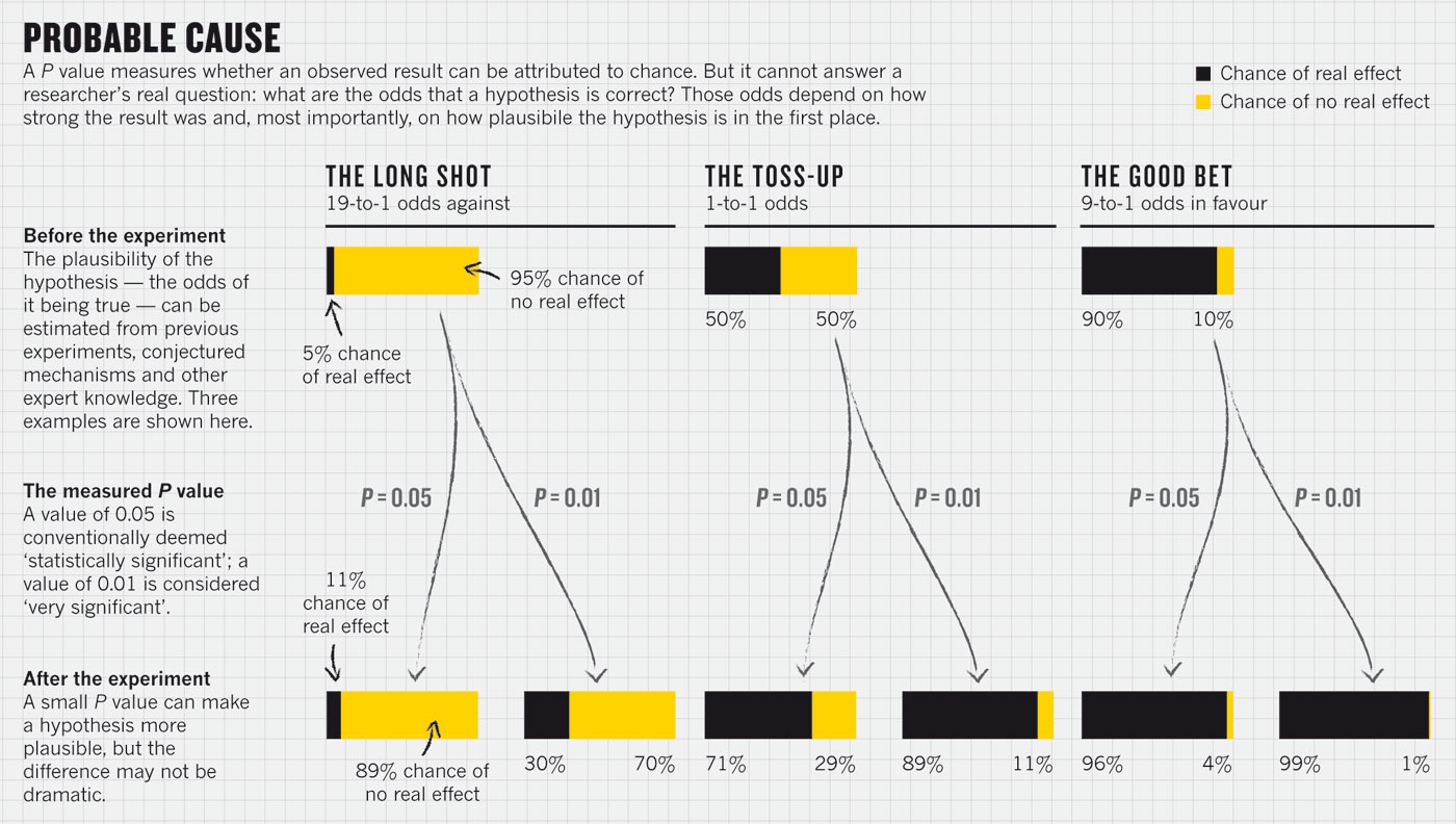
Conditional Probability and *p* = .05

A p-value = The probability of observing these data (or more extreme), given that the null hypothesis is true

  • P(D) = the probability of observing these data or more extreme data
  • P(N) = the probability that the null hypothesis is true
  • p = P(D|N)
  • But what you probably want to know is not whether these data are likely given that the null is true…
  • …but, rather, whether the null hypothesis is true or not given these data you've observed: P(N|D)

Bayes' theorem, and its notation

Bayes' Theorem is the equation that describes how a conditional probability is related to its inverse:

  • P(A|B) = P(B|A)*P(A) / P(B)
  • More generally, P(θ|D) = P(D|θ)*P(θ) / P(D)
    • “posterior = likelihood * prior / evidence”
    • P(B) = P(B|A)P(A) + P(B|Not A)P(Not A)

Examples:

  • P(ASD|male) =
    P(male|ASD) x P(ASD) / P(male) = (.811) x (.015) / (.50) = .024
  • P(male|ASD) =
    P(ASD|male) x P(male) / P(ASD) = (.024) x (.50) / (.015) = .8

Problems with NHST

The (muddled) logic of p values

  • p = P(D|N)
  • ? = P(N|D)
  • This was highlighted in a popular Nature article last year:

    infographic

Problems with NHST, cont.

Multiple comparisons

  • 30 people into 1 control group, 4 treatment groups (6 people per group). Control vs. T1 yields t = 2.95.
    Q: Is that significant?
  • RA #1: You give her the two groups. She compares the two groups. Significant!
  • RA #2: You give him all five groups, and ask for all pairwise comparisons. Correcting for familywise error, critical t is 3.43. Not significant!
  • PI: Intends to do all pairwise comparisons, but asked the first RA to just do the single comparison. Claims significance, but is planning to do multiple comparisons while using a critical t value meant for a single comparison.

Bayes doesn't care about your intentions

  • The problem with multiple comparisons in NHST arises when you try to convert a measurement of your data (the test statistic) into a probability (the p value). The mechanics of this conversion rely on a host of assumptions that may or may not be reasonable.
  • Bayesian inference skips the issue completely by never having to convert to and from probability estimates.

Clarification: Bayes vs. Frequentist

Bayesian Frequentist
Estimation HDIs, ROPEs,
posteriors
CIs,
equivalence tests
Hypothesis
Testing
BFs NHST

Clarification: Bayes vs. Frequentist

Some ideas to keep in mind…

  • Estimation approaches in general mean no uninformative results. Hooray!
  • Bayesian approaches use estimation more often, frequentist traditionally use mostly hypothesis testing (p values) - but that's about how each tool gets used, not what it's capable of.
  • You spell out your model assumptions explicitly with Bayes (although this may become less obvious as the tools become more user-friendly).

Bringing in background knowledge

  • “Updating” a prior in future research.
    • When you do Bayesian analyses, you explicitly state your prior (i.e., your background assumptions, or lack thereof) to communicate your model.
  • What might inform your prior:
    • Previous research
    • Theory-based assumption
    • (Sometimes, you don't have a well-informed prior, so you use something vague.)

We can use *Distributions* of priors!

We can use *Distributions* of priors!

Nuts and bolts

Example time!

Krushke's simple linear regression example: What is the relationship between height and weight?

Nuts and bolts

The prior!

plot of chunk unnamed-chunk-1

Nuts and bolts

The data!

plot of chunk unnamed-chunk-2

Nuts and bolts

The posterior!

plot of chunk unnamed-chunk-3

Nuts and bolts

compare to NHST correlation


    Pearson's product-moment correlation

data:  x and y
t = 4.4191, df = 28, p-value = 0.0001354
alternative hypothesis: true correlation is not equal to 0
95 percent confidence interval:
 0.3650241 0.8134220
sample estimates:
      cor 
0.6409977 

Nuts and bolts

Nuance in the results

plot of chunk ExampleNutsAndBolts

Problems Bayes won't fix for you

  • You still need to design a good experiment.
  • You still need to worry about random selection and generalizability of your results.
  • You still need a good amout of data; the more data you have, the more informative your results will be.
  • You still need to worry about experimenter degrees of freedom (although you can relax about multiple comparisons). See this blog post.

How to learn more

  • Get a good book (Kruschke, Gelman, L&W, etc.).
  • Come to Bayes Club.
  • Consider doing a summer workshop. Rose recommends the 4-week Bayes Intro at ICPSR.
  • Pester the department Powers That Be to provide us with opportunities to learn this stuff
    • Ulrich (head), Sara (GEC), Azim (chair of colloquium committee)
    • The quant profs: Lou, Robert, and Elliot (611/612/613), Sanjay (SEM), Gerard (psychometrics)
    • MethLab is a great venue for pestering (Sanjay, Elliot, and Rose)
    • Let Sara know you'd like to have a Bayesian expert come talk to us for the big data series!

Questions?

Bayesian inference elegantly incorporates background knowledge

Bayes Theorem revisited

  • P(θ|D) = P(D|θ)*P(θ) / P(D)
    • “posterior = likelihood * prior / evidence”

Silver 9-11 example:

The first plane hits

Bringing in background knowledge

The first plane hits
The second plane hits