Data 607 Project 2
Sung Lee
3/2/2020
Assignment on RPubs
Rmd on GitHub
Introduction
The purpose of this project is to work with three datasets, tidy the data, and repurpose for data analysis. The three datasets I will use are: Leo Yi’s climate data from https:/www.usclimatedata.com, Philip Tanofsky’s Coronavirus data https://github.com/CryptoKass/ncov-data/blob/master/world.latest.bno.csv, and Gehad Gad’s Academic Advising data https://raw.githubusercontent.com/logicalschema/DATA607/master/Project%202/Advising.png.
If you wish to see the R code used, there is a Code button in each section to view the code.
I will use the following R libraries.
library(stringr)
library(tidyr)
library(dplyr)
##
## Attaching package: 'dplyr'## The following objects are masked from 'package:stats':
##
## filter, lag## The following objects are masked from 'package:base':
##
## intersect, setdiff, setequal, unionlibrary(ggplot2)
library(rvest) #This R library allows you to scrap web pages## Loading required package: xml2Climate Data
The original climate data comes from https:/www.usclimatedata.com for New York-La Guardia Airport New York. I saved the page as html and saved in my GitHub account. Because the data is in HTML tables, I will scrap the data and reconstruct the data into a format that is usable. This will be done using the rvest library.
Importing
climateHTML <- read_html("https://raw.githubusercontent.com/logicalschema/DATA607/master/Project%202/usclimatedata.html")

#Read in the specific HTML nodes that have our data
climateTableOne <- html_nodes(climateHTML, "#monthly_table_one") %>% html_table()
climateTableTwo <- html_nodes(climateHTML, "#monthly_table_two") %>% html_table()
Here is a look at the imported data:
climateTableOne## [[1]]
## JanJa FebFe MarMa AprAp MayMa JunJu
## 1 Average high in ºFAv. highHi 39.00 42.00 50.00 61 71.00 80.00
## 2 Average low in ºFAv. lowLo 27.00 29.00 35.00 44 54.00 64.00
## 3 Av. precipitation in inchAv. precip.Pre. 3.17 2.76 3.97 4 3.79 3.94
## 4 Av. snowfall in inchSnowfallSn 7.00 9.00 4.00 1 0.00 0.00climateTableTwo## [[1]]
## JulJu AugAu SepSe OctOc NovNo DecDe
## 1 Average high in ºFAv. highHi 85.0 84.00 76.00 65.00 55.00 44.00
## 2 Average low in ºFAv. lowLo 69.0 69.00 62.00 51.00 42.00 32.00
## 3 Av. precipitation in inchAv. precip.Pre. 4.5 4.12 3.73 3.78 3.41 3.56
## 4 Av. snowfall in inchSnowfallSn 0.0 0.00 0.00 0.00 0.00 5.00Tidying
Let’s merge the two tables.
climateData <- merge(climateTableOne, climateTableTwo)Here is a view of the data.
climateDataLet’s rename the columns:
#Rename the columns "JanJa" "FebFe" "MarMa" "AprAp" "MayMa" "JunJu" "JulJu" "AugAu" "SepSe" "OctOc" "NovNo" "DecDe"
climateData <- rename(climateData, "Jan" = "JanJa")
climateData <- rename(climateData, "Feb" = "FebFe")
climateData <- rename(climateData, "Mar" = "MarMa")
climateData <- rename(climateData, "Apr" = "AprAp")
climateData <- rename(climateData, "May" = "MayMa")
climateData <- rename(climateData, "Jun" = "JunJu")
climateData <- rename(climateData, "Jul" = "JulJu")
climateData <- rename(climateData, "Aug" = "AugAu")
climateData <- rename(climateData, "Sep" = "SepSe")
climateData <- rename(climateData, "Oct" = "OctOc")
climateData <- rename(climateData, "Nov" = "NovNo")
climateData <- rename(climateData, "Dec" = "DecDe")
Let’s convert the month columns to rows and the rows for column Var.1 to individual columns.
#Convert the columns from Jan to Dec as row values and retain the value
climateData <- gather(climateData, key = "Month", value = "Number", "Jan":"Dec" )

#Convert the rows in the column Var.1 to column and retain the value
climateData <- spread(climateData, "Var.1", "Number")

#Rename the columns
climateData <- rename(climateData, "Av Precip" = "Av. precipitation in inchAv. precip.Pre.")
climateData <- rename(climateData, "Av Snowfall in inches" = "Av. snowfall in inchSnowfallSn")
climateData <- rename(climateData, "Av High in ºF" = "Average high in ºFAv. highHi")
climateData <- rename(climateData, "Av Low in ºF" = "Average low in ºFAv. lowLo")


#Order rows by Month
climateData <- climateData[order(factor(climateData$Month, levels = month.abb)), ]

#Order the Month column: Needed for plot
climateData$Month <- factor(climateData$Month, levels = month.abb)
Here is what the dataframe looks like now:
climateDataAnalysis
Now our data is ready for analysis. Each tab contains a different plot of the data.
This is a summary of the data:
summary(climateData)## Month Av Precip Av Snowfall in inches Av High in ºF
## Jan :1 Min. :2.760 Min. :0.000 Min. :39.00
## Feb :1 1st Qu.:3.522 1st Qu.:0.000 1st Qu.:48.50
## Mar :1 Median :3.785 Median :0.000 Median :63.00
## Apr :1 Mean :3.728 Mean :2.167 Mean :62.67
## May :1 3rd Qu.:3.978 3rd Qu.:4.250 3rd Qu.:77.00
## Jun :1 Max. :4.500 Max. :9.000 Max. :85.00
## (Other):6
## Av Low in ºF
## Min. :27.00
## 1st Qu.:34.25
## Median :47.50
## Mean :48.17
## 3rd Qu.:62.50
## Max. :69.00
## This is a summary of the differences between the Average High and Average Low Temperature each month for the set:
##    Min. 1st Qu.  Median    Mean 3rd Qu.    Max.
##    12.0    13.0    14.5    14.5    16.0    17.0
Precipitation
ggplot(climateData, aes(x=Month, y=`Av Precip`)) +
  geom_bar(alpha = .5,
           stat = "identity",
           position = position_dodge(),
           fill="blue",
           width = 0.5,
           colour="black") +
  ylim(0, 6) +
  ggtitle("Average Precipitation in Inches by Month") +
  xlab("Month") +
  ylab("Average Precipitation")
Snowfall
ggplot(climateData, aes(x=Month, y=climateData$"Av Snowfall in inches")) +
  geom_bar(alpha = .5,
           stat = "identity",
           position = position_dodge(),
           fill="azure",
           width = 0.5,
           colour="black") +
  ggtitle("Average Snowfall in Inches by Month") +
  xlab("Month") +
  ylab("Average Snowfall")
## Warning: Use of `climateData$"Av Snowfall in inches"` is discouraged. Use `Av
## Snowfall in inches` instead.
High and Low Temperature
ggplot(climateData, aes(x=Month)) +
  geom_bar(aes(y=climateData$"Av High in ºF"),
           alpha = .5,
           stat = "identity",
           position = position_dodge(),
           fill="red",
           width = 0.5,
           colour="black") +
  geom_bar(aes(y=climateData$"Av Low in ºF"),
           alpha = .5,
           stat = "identity",
           position = position_dodge(),
           fill="deepskyblue",
           width = 0.5,
           colour="black") +
  geom_bar(aes(y=climateData$"Av High in ºF" - climateData$"Av Low in ºF" ),
           stat = "identity",
           position = position_dodge(),
           fill="#056644",
           width = 0.5,
           colour="black") +
  ggtitle("Average High and Low in ºF by Month") +
  xlab("Month") +
  ylab("Temperature in ºF")
## Warning: Use of `climateData$"Av High in ºF"` is discouraged. Use `Av High in
## ºF` instead.## Warning: Use of `climateData$"Av Low in ºF"` is discouraged. Use `Av Low in ºF`
## instead.## Warning: Use of `climateData$"Av High in ºF"` is discouraged. Use `Av High in
## ºF` instead.## Warning: Use of `climateData$"Av Low in ºF"` is discouraged. Use `Av Low in ºF`
## instead.
Key:
High Temperature Low Temperature Difference between High and Low Temperature
Corona Virus Data
The original corona virus data is from https://github.com/CryptoKass/ncov-data/blob/master/world.latest.bno.csv. I saved the csv to my GitHub account. Here is the link. The csv was straightforward except for the notes column which needs to be parsed with regular expressions.
Importing
Let’s import the data from GitHub. A view of what is imported is below.
coronaCSV <- read.csv("https://raw.githubusercontent.com/logicalschema/DATA607/master/Project%202/corona.csv")
coronaCSVnames(coronaCSV)## [1] "X" "country" "cases" "deaths" "notes" "links"A note about the csv, for notes, if the value is empty, there is a 0 otherwise there will be a comma-delimited list of fields for critical, serious, and recovered.
Tidying
With the present state of the corona data, we will need to search through the coronaCSV$notes column and extrapolate new column values for critical, serious, and recovered. The initial column names are below.
newColumns <- data.frame(matrix(ncol = 3, nrow = 0))
x <- c("critical", "serious", "recovered")
names(newColumns) <- x

#Declare variables for critical, serious, and recovered
c <- 0
s <- 0
r <- 0


colnames(coronaCSV)
## [1] "X" "country" "cases" "deaths" "notes" "links"items <- coronaCSV$notes
for (row in 1:length(items)){
item <- items[row]
#If the notes is "0", create an empty row element
if (item == "0"){
newColumns <- add_row(newColumns, "critical" = 0, "serious" = 0, "recovered" = 0)
} else {
note <- unlist(str_split(item, ","))
#Obtain the critical value
p <- grep("critical", note)
if ( length(p) > 0){
tempString <- note[p]
tempString <- str_trim(str_replace(tempString, "critical", ""))
c <- as.numeric(tempString)
} else {
c <- 0
}
#Obtain the serious value
p <- grep("serious", note)
if ( length(p) > 0){
tempString <- note[p]
tempString <- str_trim(str_replace(tempString, "serious", ""))
s <- as.numeric(tempString)
} else {
s <- 0
}
#Obtain the serious value
p <- grep("recovered", note)
if ( length(p) > 0){
tempString <- note[p]
tempString <- str_trim(str_replace(tempString, "recovered", ""))
r <- as.numeric(tempString)
} else {
r <- 0
}
newColumns <- add_row(newColumns, "critical" = c,"serious" = s,"recovered" = r)
}
}
#Creating a new column to match newColumns with coronaCSV
id <- 0:25
newColumns["X"] <- id
coronaCSV <- merge(coronaCSV, newColumns)
names(coronaCSV)## [1] "X" "country" "cases" "deaths" "notes" "links"
## [7] "critical" "serious" "recovered"#Reordering the columns for coronaCSV
coronaCSV <- coronaCSV[c("X",
"country",
"cases",
"deaths",
"critical",
"serious",
"recovered",
"links",
"notes")]After tidying the data, this is the new data.
coronaCSVAnalysis
We have finished tidying up the data. Now we can conduct a simple analysis of the data for cases, deaths, critical, serious, and recovered. The data is very skewed as China has reported the largest number of cases and there are no notes about the numbers of critical, serious, and recovered cases. The lack of media does shine a glaring spotlight on China.
summary( coronaCSV %>%
           select(-links, -notes, -X)
)
## country cases deaths critical
## Australia: 1 Min. : 1.0 Min. : 0.00 Min. :0.0000
## Cambodia : 1 1st Qu.: 3.0 1st Qu.: 0.00 1st Qu.:0.0000
## Canada : 1 Median : 10.5 Median : 0.00 Median :0.0000
## China : 1 Mean : 2322.0 Mean : 52.58 Mean :0.4615
## Finland : 1 3rd Qu.: 18.0 3rd Qu.: 0.00 3rd Qu.:0.0000
## France : 1 Max. :59804.0 Max. :1365.00 Max. :8.0000
## (Other) :20
## serious recovered
## Min. :0.0000 Min. : 0.000
## 1st Qu.:0.0000 1st Qu.: 1.000
## Median :0.0000 Median : 1.000
## Mean :0.4231 Mean : 2.808
## 3rd Qu.:0.0000 3rd Qu.: 3.000
## Max. :4.0000 Max. :15.000
## Following are bar charts of the Corona data by variable broken down by country.
Cases
ggplot(coronaCSV, aes(x = country, y = cases, fill = country)) +
    geom_bar(stat = "identity", width = 0.5) +
    coord_flip() +
    theme_classic()
Deaths
ggplot(coronaCSV, aes(x = country, y = deaths, fill = country)) +
    geom_bar(stat = "identity", width = 0.5) +
    coord_flip() +
    theme_classic()
Critical
ggplot(coronaCSV, aes(x = country, y = critical, fill = country)) +
    geom_bar(stat = "identity", width = 0.5) +
    coord_flip() +
    theme_classic()
Serious
ggplot(coronaCSV, aes(x = country, y = serious, fill = country)) +
    geom_bar(stat = "identity", width = 0.5) +
    coord_flip() +
    theme_classic()
Recovered
ggplot(coronaCSV, aes(x = country, y = recovered, fill = country)) +
    geom_bar(stat = "identity", width = 0.5) +
    coord_flip() +
    theme_classic()
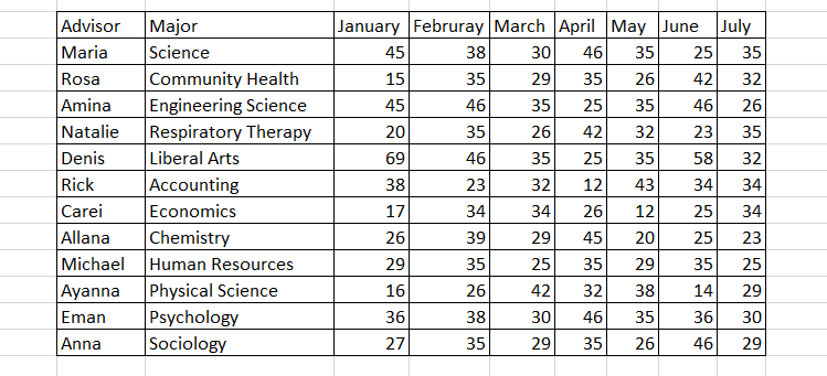
Academic Advising Data
Gehad Gad provided a data set for tidying related to academic advising. Below is a screenshot of the data.

I converted the screenshot to a csv. This csv is available at https://raw.githubusercontent.com/logicalschema/DATA607/master/Project%202/academicadvising.csv. I manually typed it but this can be done by using OCR on Acrobat or some online free website. On first view, there is no NA data. There are only 13 cases in the screenshot so I will work with these. I did have some questions about the data as I was not sure if the advisor is represented or a student that is assigned the advisor. Regardless, I will assume that the advisor listed is the actual advisor.
Importing
To begin, let’s import the Academic Advising data using the GitHub file. Here is what the initial import looks like along with the column names.
academicCSV <- read.csv("https://raw.githubusercontent.com/logicalschema/DATA607/master/Project%202/academicadvising.csv")
academicCSVnames(academicCSV)## [1] "ï..Advisor" "Major" "January" "February" "March"
## [6] "April" "May" "June" "July"Tidying
The imported data needs some cleanup to be used for analysis. The ï..Advisor column name needs to be fixed and as proposed by Gehad, we can gather the month and rank data into two new column names.
Let’s rename the ï..Advisor column.
academicCSV <- rename(academicCSV, "Advisor" = "ï..Advisor")
names(academicCSV)
## [1] "Advisor" "Major" "January" "February" "March" "April" "May"
## [8] "June" "July"Next, let’s convert the month columns to rows with a new column named Rank for storing the values.
academicCSV <- gather(academicCSV, key = "Month", value = "Rank", "January":"July")Here is what the data looks like.
academicCSVnames(academicCSV)## [1] "Advisor" "Major" "Month" "Rank"Analysis
After our data has been cleaned, we can begin analysis. Here is a general summary of the data.
summary(academicCSV %>%
           select(-Advisor, -Month)
)
## Major Rank
## Accounting : 7 Min. :12.00
## Chemistry : 7 1st Qu.:26.00
## Community Health : 7 Median :34.00
## Economics : 7 Mean :32.52
## Engineering Science: 7 3rd Qu.:36.00
## Human Resources : 7 Max. :69.00
## (Other) :42#Order the Months for plot
academicCSV$Month <- factor(academicCSV$Month, levels = month.name)Here is a breakdown of the data.
Advisor Rank
ggplot(academicCSV, aes(x = Month, y = Rank, group = Advisor, color = Advisor)) +
  geom_line() +
  geom_point() +
  theme_classic()
Major and Average Rank
Because each of the advisors is the unique advisor for the major, there is no noticeable difference from the plot for “Rank Over Time”
meanMajor <- academicCSV %>%
                  group_by(Major, Month) %>%
                  summarise_at(vars(Rank),
                        list(Average = mean))
meanMajor
ggplot(meanMajor, aes(x = Month, y = Average, group = Major, color = Major)) +
geom_line() +
geom_point() +
theme_classic()
Conclusion
R has many libraries that can help to wrangle, tidy, dice, and prepare data for analysis. Now, I have to endeavor in how to properly display the data analysis.