European Option Valuation

Harsh Baxi
April 23, 2017

Overview

The webpage European Option Valuation provides a tool valuing European call and put options using the Black-Scholes equations.

The page was created using R Markdown, Shiny and Plotly and is meant to be used in two ways:

To calculate the price of an option for a given set of inputs. Since the graph was created using Plotly, the price for a given value for the stock price can be read off the graph.
As a pedagogical tool to investigate the change in value of European options as a function of changes in various inputs.

Black-Scholes Equation For European Options

The equations below can be used to calculate the price of “vanilla” European call and put options for non-dividend paying stocks: \[ \tiny c = S_{0}N(d_{1}) - K e^{-rT}N(d_{2}) \]

\[ \tiny p = K e^{-rT}N(-d_{2}) - S_{0}N(-d_{1}) \]

\[ \tiny d_{1} = \frac{ln(S_{0}/K) + (r + \sigma^{2}/2)T}{\sigma\sqrt{T}} \]

\[ \tiny d_{2} = \frac{ln(S_{0}/K) + (r - \sigma^{2}/2)T}{\sigma\sqrt{T}} \]

where,
        c = Call Option Value
        p = Put Option Value
        \( S_0 \) = Stock Price
        K = Strike Price
        r = Risk-free Interest Rate
        T = Time to Expiry,
        \( \sigma \) = Volatility
        N() = Normal cumulative distribution function

Sample Calculation of Option Value

The following code shows how the Black-Scholes Equations are implemented in R.

# the rate, strike price, volatility and time to expiry are supplied as inputs via the Shiny controls

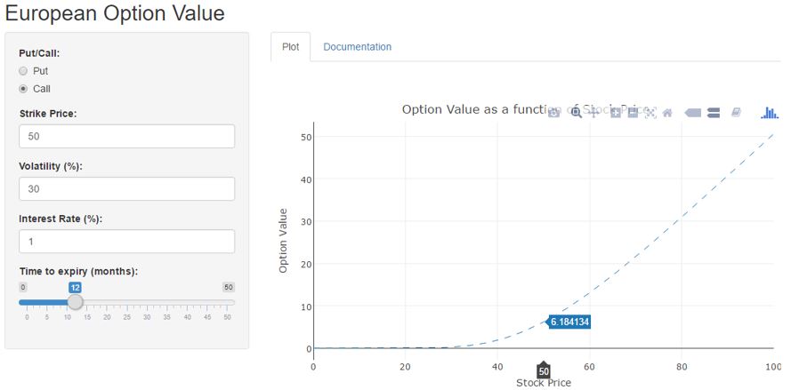
input <- data.frame("rate" = 1, "strike" = 50, volatility = 30, timeToExpiryMonths = 12, putcall = "call")

r <- input$rate / 100
k <- input$strike
v <- input$volatility / 100
t <- input$timeToExpiryMonths / 12

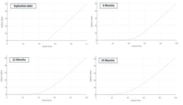
# the application calculates the option values for the range of stock prices from 0 to twice the strike price selected by the user. Here we set the stock price equal to the strike price

s <- k

# code that implements the Black-Scholes Equations

d1 <- (log(s / k) + (r + v ^ 2 / 2) * t) / (v * sqrt(t))
d2 <- (log(s / k) + (r - v ^ 2 / 2) * t) / (v * sqrt(t))

if (input$putcall == "call")
    value = s * pnorm(d1) - k * exp(-r * t) * pnorm(d2) else
    value = k * exp(-r * t) * pnorm(-d2) - s * pnorm(-d1)

print(paste("Option Value: $", round(value,2)))

[1] "Option Value: $ 6.18"

Reading the Option Value off the Plot

The option value calculated in the previous slide can be read off the graph as shown below:

Examining the trend of Option Values

The plot below shows how the webpage can be used to illustrate the effect of inputs (“Time to Expiry” in this case) on the option values: