Machine Learning on Fantasy Premier League
Introduction
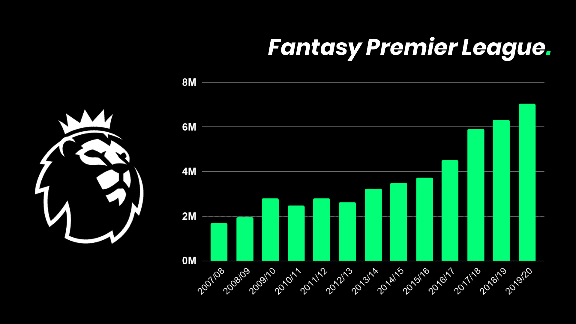
Fantasy Premier League (FPL) is a free-to-play game to choose specific combination of real life Premier League players that would contribute points based on the player’s actual statistical performance and their perceived contribution on the field of play. FPL is growing rapidly as it reaches 7 million users this season.
FPL is a unique and special because it blends the sport with the fans. It gives the fans an opportunity to manage actual Premier League players. As each player has their own assigned priced, fans need to manage their team carefully within limited budget to assemble them. In the beginning, the FPL managers would have to select 15 players, with a maximum of three players from one club. When a player on your team give you attacking contributions on the pitch like goal or assists, your team will be rewarded with points. But when your player get conceded or booked, your team suffers as well. In every round, the manager would be only given a single transfer to change their player to another players. If the manager making more than one transfer in a round, there would be point deductions for them.
Basically there are three basic ways to score points in FPL which are through events such as goals, assists and clean sheets. However the exciting part is your picked captain get the score doubled. So, whenever your captain score a goal, your FPL score will be doubled. So, your captaincy pick is crucial for your FPL team.
 “FPL user growth in the last 13 years. Source: https://fanarena.com/wp-content/uploads/2019/11/Fantasy-Premier-League-Users-per-Season.png”
For FPL managers, selecting players who would produce the most point in each round is bot easy as there are many variables that could influence. Player form may influence in some parts, but however we could not neglected other factors, such as the team overall form or the fixtures. For example, in the season of 2019/2020, Teemu Pukki from Norwich City was having an excellent form leading to the GW 6. He managed to score 49 points across five matches, including a 12-pointer against the holding champion, Manchester City! However, in the six matches afterward, amazingly he only gained 12 points.
The project aims to make a point prediction model by using machine learning. I use the dataset from fantasy.premierleague.com, understat.com and club elo.com from the 2018/2019 and 2019/2020 season from more than 150 players. The data combined from those sources giving variables such as the player form, team form, home or away fixture, Elo ratings, expected goals per 90 minutes or even the time when the match happened.
As FPL is expected to grow even faster in the future, this point prediction model would be really useful not only for fantasy premier league and football enthusiast, but also for public use.
After doing some data cleansing and wrangling which is not shown here, finally we can look into the data. The original dataset contain of 94 variables, however we would only use some of them. Let’s take a look at how Mohammed Salah of Liverpool did at the round 12-19 in season 2019/2020:
| player | round | club | opponent | was_home | total_points | goals | assists | minutes | club_elo | opponent_elo | position | value | influence_form | creativity_form | threat_form | ict_index_form | date_hour | kickoff_hour | range_day | team_scoring_form | team_conceded_form | opponent_scoring_form | opponent_conceded_form | team_form | opponent_form | fpl_form | goals_90 | assists_90 | npxG_90 | npg_90 | xG_90 | xGChain_90 | xGBuildup_90 | xA_90 | shots_90 | key_passes_90 | season | minutes_chance | scoring_chance | conceded_chance | |
|---|---|---|---|---|---|---|---|---|---|---|---|---|---|---|---|---|---|---|---|---|---|---|---|---|---|---|---|---|---|---|---|---|---|---|---|---|---|---|---|---|---|
| 6971 | Mohamed Salah | 12 | LIV | MCI | True | 8 | 1 | 0 | 86 | 2053.544 | 2025.337 | AM | 123 | 15.80 | 13.550 | 55.50 | 8.450 | 2019-11-10 16:30:00 | afternoon kick-off | 8.062 | 1.75 | 1.00 | 1.75 | 0.75 | 2.000 | 1.625 | 2.75 | 0.378 | 0.000 | 0.588 | 0.000 | 0.876 | 0.888 | 0.292 | 0.092 | 6.050 | 1.513 | 2019/2020 | 0.661 | 1.250 | 1.375 |
| 6972 | Mohamed Salah | 13 | LIV | CRY | False | 0 | 0 | 0 | 0 | 2061.503 | 1740.198 | AM | 123 | 22.55 | 4.950 | 44.00 | 7.125 | 2019-11-23 15:00:00 | afternoon kick-off | 12.938 | 2.00 | 1.00 | 0.50 | 2.00 | 2.000 | 0.375 | 4.25 | 0.769 | 0.000 | 0.359 | 0.385 | 0.652 | 0.669 | 0.327 | 0.014 | 5.385 | 0.385 | 2019/2020 | 0.650 | 2.000 | 0.750 |
| 6973 | Mohamed Salah | 14 | LIV | BHA | True | 3 | 0 | 0 | 68 | 2043.680 | 1632.715 | AM | 122 | 22.55 | 4.950 | 44.00 | 7.125 | 2019-11-30 15:00:00 | afternoon kick-off | 7.000 | 2.25 | 1.00 | 1.50 | 1.75 | 2.250 | 1.000 | 4.25 | 0.769 | 0.000 | 0.359 | 0.385 | 0.652 | 0.669 | 0.327 | 0.014 | 5.385 | 0.385 | 2019/2020 | 0.650 | 2.000 | 1.250 |
| 6974 | Mohamed Salah | 15 | LIV | EVE | True | 0 | 0 | 0 | 0 | 2044.447 | 1701.255 | AM | 122 | 11.40 | 4.300 | 28.25 | 4.375 | 2019-12-04 20:15:00 | night kick-off | 4.219 | 2.25 | 1.00 | 1.00 | 1.50 | 2.250 | 0.875 | 3.25 | 0.413 | 0.000 | 0.353 | 0.413 | 0.353 | 0.555 | 0.150 | 0.052 | 3.716 | 0.413 | 2019/2020 | 0.606 | 1.875 | 1.000 |
| 6975 | Mohamed Salah | 16 | LIV | BOU | False | 13 | 1 | 1 | 90 | 2046.424 | 1678.172 | AM | 122 | 11.40 | 4.000 | 19.50 | 3.500 | 2019-12-07 15:00:00 | afternoon kick-off | 2.781 | 3.00 | 1.25 | 1.00 | 2.00 | 2.125 | 0.000 | 2.75 | 0.584 | 0.000 | 0.324 | 0.584 | 0.324 | 0.443 | 0.046 | 0.073 | 2.922 | 0.584 | 2019/2020 | 0.428 | 2.500 | 1.125 |
| 6976 | Mohamed Salah | 17 | LIV | WAT | True | 16 | 2 | 0 | 90 | 2058.863 | 1629.378 | AM | 122 | 15.90 | 16.050 | 30.25 | 6.225 | 2019-12-14 12:30:00 | lunchtime kick-off | 6.896 | 3.00 | 1.00 | 0.25 | 1.75 | 2.250 | 0.250 | 4.00 | 0.570 | 0.570 | 0.840 | 0.570 | 0.840 | 1.097 | 0.195 | 0.434 | 3.987 | 2.848 | 2019/2020 | 0.439 | 2.375 | 0.625 |
| 6977 | Mohamed Salah | 19 | LIV | LEI | False | 3 | 0 | 0 | 69 | 2059.825 | 1826.247 | AM | 122 | 33.35 | 17.025 | 61.50 | 11.200 | 2019-12-26 20:00:00 | night kick-off | 12.312 | 3.00 | 0.75 | 2.00 | 1.25 | 2.125 | 1.375 | 8.00 | 1.089 | 0.363 | 0.894 | 1.089 | 0.894 | 1.058 | 0.124 | 0.276 | 5.081 | 1.815 | 2019/2020 | 0.689 | 2.125 | 1.375 |
I will dive into more details about variables on the above table that we’ve just read:
total_points: Our target variable. It is the point that the player gained in each specific round.club: The club where the player played.opponent: The opponent of the club.position: The position of the player on the pitch. Different with FPL terms of position, I classified it into more detail. I divided defender into two different positions, centre back (CB) and full back (FB). While, I divided midfielder into defensive midfielder (DM) and attacking midfielder (AM).value: The price of the player that set by FPL.round: The gameweek or matchweek that the game take placed.was_home: Whether the match was at home or away from the club.date_hour: The specific time where the kickoff started.kickoff_hour: Category whether the match happened at lunch, afternoon or night.range_day: The time difference between the match and the previous Premier League match.team_form: The form of the club leading to the match.opponent_form: The form of the opponent leading to the match.club_elo: The elo rating of the club leading to the match.opponent_elo: The elo rating of the opponent leading to the match.minute_chance: The number of minutes that the player have in the last 4 rounds prior to the match per 360 minutes.fpl_form: The average number of points that the player have in the last 4 rounds prior to the match.influence_form: The average number of influence rating that the player have in the last 4 rounds prior to the match.creativity_form: The average number of creativity rating that the player have in the last 4 rounds prior to the match.threat_form: The average number of threat rating that the player have in the last 4 rounds prior to the match.ict_index_form: The average number of ICT index that the player have in the last 4 rounds prior to the match.xG_90: The average number of expected goals that the player have in the last 4 rounds per 90 minutes prior to the match.xGChain_90: The average number of expected goals chain that the player have in the last 4 rounds per 90 minutes prior to the match.xA_90: The average number of expected assists that the player have in the last 4 rounds per 90 minutes prior to the match.shots_90: The average number of shots that the player have in the last 4 rounds per 90 minutes prior to the match.key_passes_90: The average number of key passes that the player have in the last 4 rounds per 90 minutes prior to the match.
Exploratory Data Analysis
One of the ways to see the relation between numeric variables is by using correlation plot. We will start by correlate team attributes such as team_form and opponent_form to our target variable:

Then, we will correlate the player attributes which contain parameters such as xG_90, fpl_form, and shots_90:

In both graph, we could say that our target variable, total_points show a weak correlation with other parameters. It shows us that we could not interpretate the player points by only using one or few variables. To predict the point, we need to combine other parameters.
The following plot is the average points of that scored by each position in each round. We could see that attacking midfielder (AM) and forward (ST) nearly dominate the highest average in every round. Forwards seem to be more fluctuative than the attacking midfielders, however they have the highest ceiling among the other positions. It also important to be noted that the full back (FB) is having a higher average points than the centre back (CB), most likely because of their attacking contributions on the picth. Defensive midfielders is the lowest among the group, that can be explained because of their lack of involvement in attack and the absence of defensive acknowledgement for them in the game.
Does the expensive player really give you more points throughout the season? If we look the following plot, the answer would be correct, generally. However, the real task is to get the best valuable player, which it means player with high points per value (or points per million). In the plot, on the high price range (right of the plot), attacking midfielders is tend to be a better value than forward throughout the season. On the lower price range, we could see that defenders from top team, such as Trent Alexander-Arnold of Liverpool or Aymeric Laporte of Man City are a better value pick than the other positions.
Which position frequently give us double digit returns in each round throughout the season? We are trying answer the question by using the following graph. The left one is the number of single digit returns (6 - 9 points) that produced by position in each round and the right is the double digit returns (> 9 points). From the graph it is obvious that only full back and attacking midfielder that give us consistent number of single digit return of more than 150 times. However only attacking midfielder that give us more than 100 times of double digit returns throughout the season.

In the following plot, we would like to know if club influenced the points gained by player. On the plot, we compare average (yellow dot) and the maximum points (blue dot) that can be achieved by the player from each clubs. Top rank clubs like Liverpool and Manchester City as expected generates high average points and also having a high ceiling than other clubs. Watford shows us that their players could gain high points in one or few rounds although the points will be normalized into the average throughout the season.

Machine Learning Model
Random Forest
Random forest is a Supervised Learning algorithm which uses ensemble learning method for classification and regression. In order to prevent bias in our model, we remove the data under 0.1% in our target variable, so that our target variable will range from -2 to 16.
## .
## -6 -4 -3 -2 -1 0
## 0.01355197 0.01355197 0.04065592 0.20327958 0.71825451 21.12752405
## 1 2 3 4 5 6
## 17.44138772 27.30722320 6.84374577 1.55847676 3.52351267 7.26385689
## 7 8 9 10 11 12
## 3.26602521 2.81881014 2.49356281 1.27388535 0.93508606 0.90798211
## 13 14 15 16 17 18
## 0.67759859 0.37945521 0.52852690 0.27103944 0.09486380 0.06775986
## 19 20 21 23 24
## 0.06775986 0.06775986 0.06775986 0.01355197 0.01355197Before do the modeling, we need to do cross validation. We seperate the data into training and test dataset.
set.seed(100)
splitted <- rsample::initial_split(fpl_ml_rm, 0.7, "total_points")
fpl_train <- rsample::training(splitted)
fpl_test <- rsample::testing(splitted)fpl_train <- fpl_train %>%
dplyr::select(- c(player, round, goals, assists, minutes, date_hour, season))
fpl_test <- fpl_test %>%
dplyr::select(- c(player, round, goals, assists, minutes, date_hour, season))Then we can start the modeling:
Neural Network/Deep Learning
Neural networks are set of algorithms that comprised of an arrangement of “layers” and “nodes” (representing neurons) such that “information” flows from one later and relayed to another, which designed to recognize patterns.
Before modeling, we divided the data in train and test data for ratio of 7:3.
fpl_ml <- read.csv("fpl_ml.csv")
fpl_ml_rm <- fpl_ml %>%
dplyr::filter(total_points < 16 & total_points > -2) %>%
dplyr::select(- X)
set.seed(100)
splitted <- rsample::initial_split(fpl_ml_rm, 0.7, "total_points")
fpl_train <- rsample::training(splitted)
fpl_test <- rsample::testing(splitted)train_x_keras <- model.matrix(~club + opponent + was_home + club_elo + opponent_elo + position + value + influence_form + creativity_form + threat_form + threat_form + ict_index_form +
kickoff_hour + range_day + team_form + opponent_form + fpl_form +
goals_90 + assists_90 + xG_90 + xGChain_90 + xGBuildup_90 + xA_90 + shots_90 + key_passes_90 + minutes_chance + scoring_chance + conceded_chance, train_x)test_x_keras <- model.matrix(~club + opponent + was_home + club_elo + opponent_elo + position + value + influence_form + creativity_form + threat_form + threat_form + ict_index_form +
kickoff_hour + range_day + team_form + opponent_form + fpl_form +
goals_90 + assists_90 + xG_90 + xGChain_90 + xGBuildup_90 + xA_90 + shots_90 + key_passes_90 + minutes_chance + scoring_chance + conceded_chance, test_x)train_x_keras <- array_reshape(train_x_keras, dim = dim(train_x_keras))
test_x_keras <- array_reshape(test_x_keras, dim = dim(test_x_keras))
train_y_keras <- train_yNow we do the modeling. We created two layers with 64 nodes at the beginning:
model %>%
layer_dense(units = 64, input_shape = ncol(train_x_keras), activation = "linear", name = "1") %>%
layer_dense(units = 32, activation = "linear", name = "2") %>%
layer_dense(units = 16, activation = "linear", name = "3") %>%
layer_dense(units = 1, activation = "linear", name = "output")Evaluation
For evaluation, there are many parameters, one of them is Mean Absolute Error (MAE). We will seperate the evaluation for data test and data train to see whether the our model is overfitting:
Random Forest
## [1] 1.89482## [1] 2.000539For the data train, we have 1.89 of MAE while for data test, the MAE is 2.00. The small differences in MAE betwen data train and data test show that our model is not overfitting. Our data has range from -2 to 16, so that MAE of 2.00 shows that our model has percentage error of 2/(16-(-2)) = 11.11%
Neural Network
## [1] 2.048037## [1] 2.078562In our neural network model, the MAE is 2.34 for the data train, while MAE is 2.41 for data test. Our data has range from -2 to 16, so that MAE of 2.41 shows that our model has percentage error of 2/(16-(-2)) = 13.39%
Conclusion
In our case, random forest proof to be perform marginally better by 0.4 than neural networkmore accurate in predicting than neural network in our dataset by 0.4. Neural networks works better when there are invariants to the data such as for the case in image recognition. However, when these invariances do not exist, they do not have much of an advantage.