• 1. Introduction of Monte Carlo
  
  

• 2. Random Number Generation
  
  

• 3. Variance Reduction
  
  

• 4. Metropolis Algorithm
  
  

• 5. Simulated Annealing Algorithm(SAA)
  
  

• 6. Quasi-Monte Carlo Method

Monte Carlo is a famous casino in Monaco(Europe). During the Second World War, Metropolis used its name to nominate a certain kind of numerical method.

• Main advantage: describe the whole system directly, rather than the evolution process(ODE, PDE, SDE)
  
  

• Example: Statistical physics
  

  We want to know the macro-level properties of massive particles, like temperature, it essentially an expectation from phase space:

  \[\int...\int f(\mathbf x)d\mathbf x\] It’s impossible to use traditional method to solve it(“curse of dimension”).

We take one dimension to compare the MC and traditional method. \[I(f) = \int_0^1 f(x)dx\] (1) Traditional Method: \[I(f) \approx [\frac{1}{2}f(x_0) + \sum_{i=1}^{N-1}f(x_i) + \frac{1}{2}f(x_N)]h\] \[h= \frac{1}{N}, x_i = ih\]

(2) Monte Carlo Method: \(I(f) = Ef(x)\), according to the Law of Large Number \[I(f) \approx \frac{1}{N}\sum_{i=1}^{N}f(X_i) = I_N(f), X_i \sim U(0, 1)\]

• Let’s show \(I(N)\) converges to \(I(f)\): \[EI_N(f) = E[\frac{1}{N}\sum_{i=1}^{N}f(X_i)] = \frac{1}{N}\sum_{i=1}^{N}\int_0^1f(x)dx=I(f)\]
• The error \(e_N\) is a random variable, let’s estimate the square error: \[\begin{split} E|e_N|^2=E[I_N(f)-I(f)]^2=E[\frac{1}{N}\sum_{i=1}^{N}(f(X_i)-I(f))]^2 \\ =\frac{1}{N^2}\sum_{i,j=1}^{N}E[f(x_i)-I(f)][f(x_j)-I(f)]\\ =\frac{1}{N}E[f(x_i)-I(f)]^2=\frac{1}{N}Var(f) \end{split} \]

\[E|e_N|\leq \sqrt{E|e_N|^2}=\frac{\sqrt{Var(f)}}{\sqrt{N}} \]

Note: If \(f\) has finite variance, then MC has a \(\frac{1}{2}\)-order convengency(to be improved later)

MC is totally based on random number, so how to efficiently generate random number that following a specific distribution?

Pseudo-random number, which generate numbers that look random, but are actually deterministic, and can be reproduced if the state of the generator is known.

• Content

• 2.1 The generation of uniform distribution
  

• 2.2 The generation of more general distribution

  • Transformation method
  • Box-Muller(Normal Distribution)
  • Acceptance-rejection method
  • Other method

Note: it is dangerous to directly apply a poor random number generator into encryption.

Linear congruential algorithm(frequently used)

线性同余法 \[X_{n+1}=[aX_{n}+c] mod[m] \\ a, c, m \in N\]

1. \(m=2^{31}-1\) for 32-bit computer
2. \(a\) is multiplier
3. \(c\) is increment
4. \(X_0\) is initial seed \[U_n=X_n/m\]

• Measurement: Cycle Length
  
  • the longer, the better
  • \(m\) is the largest cycle length.

If random variable Y has \(CDF\space F(y)\), if \(X\sim U(0,1)\), then \(Y=F^{-1}(X)\) is the desired distribution.

• \(Proof:\) \[X\sim U(0,1), Y=F^{-1}(X)\\ P(Y\leq y) = P(F^{-1}(X)\leq y)=P(X\leq F(y))=F(y) \]

• Example:\[p(y)= \begin{cases} \lambda e^{-\lambda y}, Y!=f(x) \\ 0, \space \space \space \space \space \space \space y \leq 0 \end{cases} \] \[F(y)=\int_0^yp(z)dz=1-e^{-{\lambda y}}\\ F^{-1} (x) = -\frac{1}{\lambda}ln(1-x), x \in (0,1)\\ Y_i = -\frac{1}{\lambda}ln(1-X_i) \]

To get normal distribution, we use the integration technique:
\[Question: \int_{-\infty}^{\infty} e^{-x^2}dx \\ (\int_{-\infty}^{\infty} e^{-x^2}dx)^2=\int_{-\infty}^{\infty} \int_{-\infty}^{\infty} e^{-(x^2+y^2)}dxdy=\int_0^{\infty} \int_0^{2\pi} e^{-r^2}rdrd{\theta} =\pi \] Box-Muller: \[(x_1, x_2)=(rcos\theta,rsin\theta)\\ \frac{1}{2\pi}e^{-\frac{x_1^2+x_2^2}{2}}dx_1dx_2=\frac{1}{2\pi}e^{-\frac{r^2}{2}}rdrd\theta\\ =(\frac{1}{2\pi}d\theta)(e^{-\frac{r^2}{2}}rdr) \]

then, use transformation method \(\theta=2\pi U_1, R=\sqrt{-2ln(1-U_2)}=\sqrt{-2lnU_2^{'}}\)
\[X_1=Rcos\theta=\sqrt{-2lnU_2^{'}}cos(2\pi U_1)\]

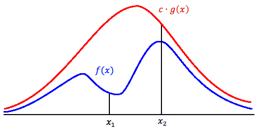
Suppose \(X, Y\) are random variables, they have \(pdf \space f, g \space respectively\). This algorithm has these steps:

1. find a \(r.v. Y with\space \frac{f(t)}{g(t)}\leq c\)
2. generate a number \(y\) from \(g\)
3. generate a number \(u\) from \(U(0, 1)\)
4. if \(u \leq \frac{f(y)}{cg(y)}\), then accept \(x=y\), reject \(y\) otherwise.
5. repeat 2-4 until we have enough points

\(Proof:\)
We only need to proof \(P(Y\leq y|U \leq \frac{f(t)}{cg(t)})=F_X(y)\)

\[P(Y\leq y|U \leq \frac{f(Y)}{cg(Y)})=\frac{P(Y\leq y, U \leq \frac{f(Y)}{cg(Y)})}{1/c}\\ =\int_{-\infty}^y \frac{P(U \leq \frac{f(Y)}{cg(Y)}|Y=w\leq y)}{1/c}g(w)dw\\ =c\int_{-\infty}^y\frac{f(w)}{cg(w)}g(w)dw=F_X(y) \]

Advantage: computation time is invariant with \(x\)

• If \(Z \sim N(0,1), then \space Z^2 \sim {\chi}^2(1)\)

• If \(U \sim {\chi}^2(m), V \sim {\chi}^2(n), then \space F=\frac{U/m}{V/n} \sim F(m,n)\)

• If \(Z \sim N(0,1), V \sim {\chi}^2(n), then \space T=\frac{z}{\sqrt{V/n}} \sim t(n)\)

3.1 Importance Sampling (Intuition: A change of variable/measure)

• Sampling from known distribution \(q(x)\),
  we have \(I=\int f(x)\pi(x)dx = \int f(x) \frac{\pi(x)}{q(x)}q(x)dx\) \[Importance: W(x) = \frac{\pi(x)}{q(x)}\]
• Importance Sampling uses another distribution \(q(x)\) to reduce the variance. We take \(\pi(x)=1, which \space means \space X \sim U(0,1)\)

\[I(f)=\int_0^1f(x)dx=\int_0^1\frac{f(x)}{q(x)}q(x)dx\\ \int_0^1q(x)=1\\ I(f) \approx \frac{1}{N}\sum_{i=1}{N}\frac{f(Y_i)}{q(Y_i)} \]

• Variance analysis \[Var_X(f)=\int_0^1[f-I(f)]^2dx=\int_0^1f^2dx-I^2(f)\\ Var_Y(\frac{f}{q})=\int_0^1(\frac{f}{q})^2qdy-I^2(f)=\int_0^1\frac{f^2}{q}dy-I^2(f) \]

• If we choose suitable \(q(x)\), let \[\int_0^1\frac{f^2}{q}dy \leq \int_0^1f^2dx\] the variance will be reduced.

(Intuition: use the linearity of integral)

\[\int f(x)dx=\int [f(x)-g(x)]dx+\int g(x)dx\]

• Requirements for \(g(x):\)

  • \(\int g(x)dx\) is can be obtain accurately
  • the variance of \(\int [f(x)-g(x)]dx\) is smaller than \(\int f(x)dx\)

Intuition: the random numbers are i.i.d, but if we can generate negatively correlated random numbers, we will reduce the variance.

• Example: \(\int_0^1 f(x)dx\)
  • generate \(X_i\sim U(0, 1)\)
  • calculate \([\frac{f(x_i)+f(1-x_i)}{2}]\)
  • get \(I\approx\frac{1}{N}\sum_{i=1}^{N}\frac{f(x_i)+f(1-x_i)}{2}\)
• \[EI_N=I(f)\\ Var(I_N)=\frac{1}{2N}[Var(f)+Cov(f(X), f(1-X))]\leq \frac{1}{2N}Var(f)\]