1. Open the repo at https://github.com/dlab-berkeley/Geospatial-Fundamentals-in-R-with-sf
   • Clone the repo or download and unzip the zip file
   • Take note of the folder in which the files are located

2. Start RStudio and open a new script, or ./docs/01-core_concepts_and_plotting.Rmd

3. Set your working directory to the folder you unzipped

4. Install the required libraries in RStudio, if you do not have them already

install.packages(
  c("ggplot2", "dplyr", "sf", "units", "tmap", "nngeo", "raster"),
  dependencies=TRUE)
}

1. Open the slides, ./docs/01-core_concepts_and_plotting.Rmd, in your browser (or click the “Part 1 Slides” link the repo).

Who are you?

Why are you here?

You have options:

1. Open the slides in your browser (click on the link in the repo, or launch from your local copy of the HTML file).

2. Open the Rmd script (or a blank script) in RStudio.

3. Both of the above.

4. Just chill and watch.

Slides ./docs/01-core-concepts-and-plotting.html

RMarkdown Code ./docs/01-core-concepts-and-plotting.Rmd

Make sure you can cut and paste into RStudio

Intro to working with geospatial data in R

• Geospatial data files and formats
• Loading geospatial data in R
• R packages for working with geospatial data
• Coordinate reference systems & map projections
• Mapping geospatial data

Key goal is familiarity, competency takes lots of practice

are data with locations on or near the surface of the Earth.

represent location more specifically with coordinates

46.130479, -117.134167

Coordinates only make sense when associated with a CRS!

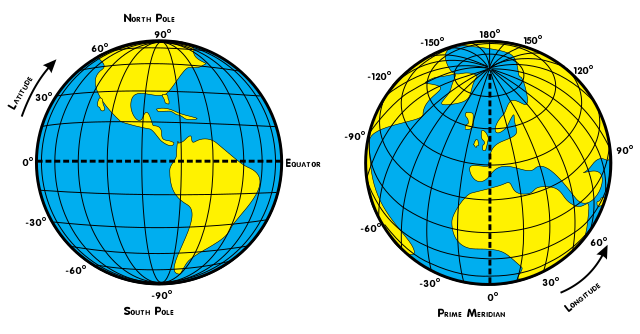
Geographic Coordinates: Latitude and Longitude

Define:

• the shape of the Earth

• the origin (0,0 point)

• the relationship between the system and the real world

• the units

Because of variations in these, there are many geographic CRSs!

The World Geodetic System of 1984 is the most widely used geographic coordinate reference system.

WGS84 is the default CRS for most GIS software

Almost all longitude and latitude data are assumed to be WGS84 unless otherwise specified

Historical data much trickier

You can

• dynamically determine spatial metrics like area, length, distance and direction

• spatial relationships like intersects, inside, contains, etc

and

• link data by location, like census data and crime data

Spatial data is a broader term than geographic data.

Methods for working with spatial data are valid for geospatial data

All spatial data are encoded with some type of coordinate reference system

Geospatial data require the CRS to be a model of locations on the Earth

Vector and Raster Data

Points, lines and Polygons

Regular grid of cells (or pixels)

We cover raster data only in Day 3 of this workshop

software that can import, create, store, edit, visualize and analyze geospatial data

• represented as geometric data objects referenced to the surface of the earth via CRSs

• with methods to operate on those representations

We call software for working with geospatial data GIS

Geographic Information System

This term is commonly associated with desktop software applications.

Desktop GIS - ArcGIS, QGIS

Spatial Databases - PostgreSQL/PostGIS

Web-based GIS - ArcGIS Online, CARTO

Software geospatial data support - Tableau

Programming languages with geospatial data support

• R, Python, Javascript

You already use R

Reproducibility

Free & Open Source

Strong support for geospatial data and analysis

Cutting edge

Make sure you have set your working directory to the location of the workshop files.

Make sure you have the packages we are going to use installed.

#
# Geospatial Data in R Workshop
#

# Make sure needed packages are installed
our_packages<- c("ggplot2", "dplyr", "sf", "units", "tmap", "raster", "nngeo")

for (i in our_packages){
  if ( i %in% rownames(installed.packages()) == FALSE) {
    print(paste(i, "needs to be installed!"))
    install.packages(i)
    
  } else {
    print(paste0(i, " [", packageVersion(i), "] is already installed!"))
    
  } 
}

# Set working directory to folder with workshop files
#setwd("~/Documents/Dlab/workshops/2019/Geospatial-Fundamentals-in-R-with-sf")

There are many approaches to and packages for working with geospatial data in R.

One approach is to keep it simple and store geospatial data in a data frame.

This approach is most common when

• the data are point data in CSV files and

• you want to map rather than spatially transform or analyze the data

sf_properties_25ksample.csv

San Francisco Open Data Portal https://data.sfgov.org

SF Property Tax Rolls

This data set includes the Office of the Assessor-Recorder’s secured property tax roll spanning from 2007 to 2016.

We are using a subset of these data as a proxy for home values.

SFhomes <- read.csv('/Users/dr.auwal/Desktop/Personals/UC Berkeley/Workshops/Geospatial-Fundamentals-in-R-with-sf/2nd Workshop/Geospatial-Fundamentals-in-R-with-sf-master/data/sf_properties_25ksample.csv', 
                    stringsAsFactors = FALSE)

# Take a look at first 5 rows and a few of the columns
SFhomes[1:5,c("YearBuilt","totvalue","AreaSquareFeet","Neighborhood",
              "NumBedrooms")]

Make sure your working directory is set to the folder where you downloaded the workshop files!

SFhomes <- read.csv('/Users/dr.auwal/Desktop/Personals/UC Berkeley/Workshops/Geospatial-Fundamentals-in-R-with-sf/2nd Workshop/Geospatial-Fundamentals-in-R-with-sf-master/data/sf_properties_25ksample.csv', 
                    stringsAsFactors = FALSE)

# Take a look at first 5 rows and a few of the columns
SFhomes[1:5,c("YearBuilt","totvalue","AreaSquareFeet","Neighborhood",
              "NumBedrooms")]

##   YearBuilt totvalue AreaSquareFeet       Neighborhood NumBedrooms
## 1      1923  1031391           2250 West of Twin Peaks           0
## 2      1909   775300           5830   Presidio Heights           3
## 3      1915  1116772           1350     Inner Richmond           2
## 4      1947   860130           1162    Sunset/Parkside           0
## 5      1981   322749           1463     Outer Richmond           3

class(SFhomes)            # what is the data object type?
dim(SFhomes)              # how many rows and columns
str(SFhomes)              # display the structure of the object
head(SFhomes)             # take a look at the first 10 records
summary(SFhomes)          # explore the range of values
summary(SFhomes$totvalue) # explore the range of values for one column
hist(SFhomes$totvalue)    # histogram for the totvalue column

• What columns contain the geographic data?
• Are these data vector or raster data?
• What type of geometry do the data contain?
  • Points, lines, polygons, grid cells?
• What is the CRS of these data?

Use the R base plot function to create a simple map

plot(SFhomes$lon, SFhomes$lat) # using base plot function

Use the R base plot function to create a simple map

plot(SFhomes$lon, SFhomes$lat) # using base plot function

Most widely used plotting library in R

Not specifically for geospatial data

But can be used to make fabulous maps

Great choice if you already know ggplot2

Load the library

library(ggplot2)

Basic map with ggplot

library(ggplot2)

ggplot() + geom_point(data=SFhomes, aes(lon,lat))

Basic map with ggplot

ggplot() + geom_point(data=SFhomes, aes(lon,lat), size=1)

ggplot() + geom_point(data=SFhomes, aes(lon,lat), size=1) + coord_map()

Allows you to associate a map projection with geographic coord data.

Map Projection: mathematial transformation from curved to flat surface

A Projected CRS applies a map projection to a Geographic CRS

All introduce distortion,

• in shape, area, distance, direction, or combo

• the larger the area the greater the distortion

No one map projection best for all purposes

Selection depends on location, extent and purpose

Mercator is the default map projection used by the get_coord() function.

• You don’t have to specify it!

It’s important to know that you can customize the map projection and parameters if you wish.

But doing this is beyond the scope of this workshop.

Data driven symbology

ggplot() + geom_point(data=SFhomes, aes(lon,lat, col=totvalue)) + 
  coord_map()

What’s happening here?

SFhomes_low2high <- SFhomes[order(SFhomes$totvalue, decreasing = FALSE),]

ggplot() + 
  geom_point(data=SFhomes_low2high, aes(lon,lat, col=totvalue)) + 
  coord_map()

Try it - Does the output map look different from previous one?

The order of the data in the data frame changes the map display!

What does this code do?

SFhomes2010_15 <- subset(SFhomes_low2high, as.numeric(SalesYear) > 2009)

ggplot() +
  geom_point(aes(lon, lat, col=totvalue), data = SFhomes2010_15 )  +
  facet_wrap(~ SalesYear)

Visual spatial analysis!

Let’s add another geospatial data layer to our map.

You can use this method to add as many layers as you want to a ggplot.

Map overlay is the fundamental technique of visual geographical analysis.

Use the read.csv function to read in a file of Bart Station locations. What is the name of the column with the longitude values? latitude?

bart <- read.csv("/Users/dr.auwal/Desktop/Personals/UC Berkeley/Workshops/Geospatial-Fundamentals-in-R-with-sf/2nd Workshop/Geospatial-Fundamentals-in-R-with-sf-master/data/bart.csv")

# take a look
head (bart)

##           X        Y             STATION OPERATOR DIST  CO
## 1 -122.2833 37.87406      NORTH BERKELEY     BART    4 ALA
## 2 -122.2682 37.86969   DOWNTOWN BERKELEY     BART    4 ALA
## 3 -122.2701 37.85321               ASHBY     BART    4 ALA
## 4 -122.2518 37.84451           ROCKRIDGE     BART    4 ALA
## 5 -122.2671 37.82871           MACARTHUR     BART    4 ALA
## 6 -122.2684 37.80808 19TH STREET/OAKLAND     BART    4 ALA

For the maps from here on out, to deal with a smaller example dataset, we’re going to also subset our data for only those rows that pertain to year 2015.

SFhomes15 <- subset(SFhomes_low2high, as.numeric(SalesYear) == 2015)

sfmap_with_bart <- ggplot() +
  geom_point(data=SFhomes15, aes(x=lon, y=lat, col=totvalue))  +
  geom_point(data=bart, aes(x=X,y=Y), col="red", size=3) 

sfmap_with_bart

Let’s just display SF BART Stations

sfmap_with_bart <- ggplot() +
  geom_point(data=SFhomes15, aes(x=lon, y=lat, col=totvalue))  +
  geom_point(data=bart[bart$CO=='SF',], aes(x=X,y=Y), col="red", size=3) 

Are the higher valued homes near BART?

sfmap_with_bart

What could we do to improve our map?

sfmap_with_bart

SF Landmarks

data/landmarks.csv

landmarks <- read.csv("/Users/dr.auwal/Desktop/Personals/UC Berkeley/Workshops/Geospatial-Fundamentals-in-R-with-sf/2nd Workshop/Geospatial-Fundamentals-in-R-with-sf-master/data/landmarks.csv")
head(landmarks)

##           X       Y id             name
## 1 -13626151 4551548  1       Coit Tower
## 2 -13630804 4544523  2       Twin Peaks
## 3 -13627654 4548289  3        City Hall
## 4 -13635101 4546904  4 Golden Gate Park

Let’s create a map of the SF homes, BART Stations and Landmarks all together.

sfmap_bart_landmarks <- ggplot() +
  geom_point(data=SFhomes15, aes(x=lon, y=lat))  +
  geom_point(data=bart[bart$CO=='SF',], aes(x=X,y=Y), col="red", size=3) +
  geom_point(data=landmarks, aes(x=X,y=Y), shape=22, 
             col="black", fill="grey", size=4)

All good - are all layers displayed? If not, why not?

There are limits to what you can do with geospatial data stored in a data frame.

• i.e. where there is no specific geospatial data object(s)

head(landmarks)

##           X       Y id             name
## 1 -13626151 4551548  1       Coit Tower
## 2 -13630804 4544523  2       Twin Peaks
## 3 -13627654 4548289  3        City Hall
## 4 -13635101 4546904  4 Golden Gate Park

The Landmark data do not have geographic coordinates - longitude and latitude.

You can’t transform these coordinate data with ggplot.

ggplot() +
  geom_point(data=landmarks, aes(x=X,y=Y), shape=22, 
             col="black", fill="grey", size=4)

The ESRI Shapefile is the most common file format for geospatial data.

ggplot cannot directly read in or plot shapefile data.

• though you can do it with a round-about set of commands :(

ggplot can’t answer questions like

• What properties are in the Noe Valley neighborhood?

• What is the average property value in each SF neighborhood?

• What is the area of each SF Neighborhood and the property density?

• What properties are within walking distance (.25 miles) of the Mission neighborhood?

You need libaries that support spatial data objects and spatial methods for that!

sf stands for ‘simple features’, which is a standard (developed by the Open Geospatial Consortium) for storing various geometry types in a hierarchical data model.

A ‘feature’ is just a representation of a thing in the real world (e.g. a building, a city…).

In other words, each feature consists of both a geometric representation of an object and some associated information (building: height, name, etc…, city: population, area, etc…).

sf is a relatively new package.

sf supersedes the package sp and its ecosystem of related packages (mainly rgeos and rgdal). As such, it is a one-stop shop for core geospatial data objects and operations that used to be spread across those 3 packages.

sp is still frequently used, but its spatial objects are a bit less streamlined. It will be necessary for our raster work on Day 3, so we’ll see a bit of it then.

Here are the most common simple features geometries, which are used to represent vector data in sf.

Point Linestring Polygon Multipoint MultiLinestring MultiPolygon Geometry Collection

(From the Geocomputation in R textbook, Chapter 2, Figure 2.2)

sf offers numerous specific benefits, including:

• fast IO (Input and Output)
• enhanced plotting
• integration with R data structures (it uses data.frames)
• integration with tidyverse packages, %>% piping syntax
• consistent function names (all starting with st_ for spatial type)
• increasingly supported by other geospatial packages (e.g. tmap, ggplot)
• aligned with other GIS software that use simple features (e.g. QGIS, PostGIS) or a similar data model (e.g. Python’s Geopandas)

First, of course, we’ll need to load the package:

library(sf)

## Linking to GEOS 3.7.2, GDAL 2.4.2, PROJ 5.2.0

We can then read in a spatial dataset into an sf object using the st_read function.

Let’s start with a shapefile of San Francisco census tracts.

First take a look at the file…

dir("/Users/dr.auwal/Desktop/Personals/UC Berkeley/Workshops/Geospatial-Fundamentals-in-R-with-sf/2nd Workshop/Geospatial-Fundamentals-in-R-with-sf-master/data", pattern = "sftracts.")

## [1] "sftracts_wpop.dbf" "sftracts_wpop.prj" "sftracts_wpop.shp"
## [4] "sftracts_wpop.shx" "sftracts.dbf"      "sftracts.prj"     
## [7] "sftracts.shp"      "sftracts.shx"

Now let’s use the sf function st_read to load the file in R.

tracts = st_read(dsn = '/Users/dr.auwal/Desktop/Personals/UC Berkeley/Workshops/Geospatial-Fundamentals-in-R-with-sf/2nd Workshop/Geospatial-Fundamentals-in-R-with-sf-master/data', layer = 'sftracts')

## Reading layer `sftracts' from data source `/Users/dr.auwal/Desktop/Personals/UC Berkeley/Workshops/Geospatial-Fundamentals-in-R-with-sf/2nd Workshop/Geospatial-Fundamentals-in-R-with-sf-master/data' using driver `ESRI Shapefile'
## Simple feature collection with 195 features and 8 fields
## geometry type:  MULTIPOLYGON
## dimension:      XY
## bbox:           xmin: -13638250 ymin: 4538276 xmax: -13617440 ymax: 4560139
## epsg (SRID):    NA
## proj4string:    +proj=merc +lon_0=0 +lat_ts=0 +x_0=0 +y_0=0 +a=6378137 +b=6378137 +units=m +no_defs

Then, as always, we can explore the basic aspects of the object returned, using base R functions:

#the object displays a compact summary, when its name is called
tracts

## Simple feature collection with 195 features and 8 fields
## geometry type:  MULTIPOLYGON
## dimension:      XY
## bbox:           xmin: -13638250 ymin: 4538276 xmax: -13617440 ymax: 4560139
## epsg (SRID):    NA
## proj4string:    +proj=merc +lon_0=0 +lat_ts=0 +x_0=0 +y_0=0 +a=6378137 +b=6378137 +units=m +no_defs
## First 10 features:
##    STATEFP COUNTYFP TRACTCE             AFFGEOID       GEOID   NAME LSAD
## 1       06      075  035202 1400000US06075035202 06075035202 352.02   CT
## 2       06      075  042601 1400000US06075042601 06075042601 426.01   CT
## 3       06      075  047801 1400000US06075047801 06075047801 478.01   CT
## 4       06      075  060502 1400000US06075060502 06075060502 605.02   CT
## 5       06      075  980200 1400000US06075980200 06075980200   9802   CT
## 6       06      075  018000 1400000US06075018000 06075018000    180   CT
## 7       06      075  012501 1400000US06075012501 06075012501 125.01   CT
## 8       06      075  015200 1400000US06075015200 06075015200    152   CT
## 9       06      075  026403 1400000US06075026403 06075026403 264.03   CT
## 10      06      075  032901 1400000US06075032901 06075032901 329.01   CT
##      ALAND                       geometry
## 1   372758 MULTIPOLYGON (((-13637736 4...
## 2   293133 MULTIPOLYGON (((-13634865 4...
## 3   476606 MULTIPOLYGON (((-13636354 4...
## 4   276334 MULTIPOLYGON (((-13628231 4...
## 5  1022568 MULTIPOLYGON (((-13637838 4...
## 6   937021 MULTIPOLYGON (((-13626895 4...
## 7   135257 MULTIPOLYGON (((-13627070 4...
## 8   279195 MULTIPOLYGON (((-13629456 4...
## 9   379382 MULTIPOLYGON (((-13626769 4...
## 10  671900 MULTIPOLYGON (((-13636086 4...

What sort of object is this?

class(tracts)

# the object is of both the 'sf' and 'data.frame' classes
class(tracts)

## [1] "sf"         "data.frame"

It has a number of columns (i.e. attributes, fields), including a geometry column

str(tracts)

## Classes 'sf' and 'data.frame':   195 obs. of  9 variables:
##  $ STATEFP : Factor w/ 1 level "06": 1 1 1 1 1 1 1 1 1 1 ...
##  $ COUNTYFP: Factor w/ 1 level "075": 1 1 1 1 1 1 1 1 1 1 ...
##  $ TRACTCE : Factor w/ 195 levels "010100","010200",..: 164 169 178 184 191 70 26 42 129 155 ...
##  $ AFFGEOID: Factor w/ 195 levels "1400000US06075010100",..: 164 169 178 184 191 70 26 42 129 155 ...
##  $ GEOID   : Factor w/ 195 levels "06075010100",..: 164 169 178 184 191 70 26 42 129 155 ...
##  $ NAME    : Factor w/ 195 levels "101","102","103",..: 164 169 178 184 191 70 26 42 129 155 ...
##  $ LSAD    : Factor w/ 1 level "CT": 1 1 1 1 1 1 1 1 1 1 ...
##  $ ALAND   : num  372758 293133 476606 276334 1022568 ...
##  $ geometry:sfc_MULTIPOLYGON of length 195; first list element: List of 1
##   ..$ :List of 1
##   .. ..$ : num [1:9, 1:2] -13637736 -13636969 -13636954 -13636940 -13636925 ...
##   ..- attr(*, "class")= chr  "XY" "MULTIPOLYGON" "sfg"
##  - attr(*, "sf_column")= chr "geometry"
##  - attr(*, "agr")= Factor w/ 3 levels "constant","aggregate",..: NA NA NA NA NA NA NA NA
##   ..- attr(*, "names")= chr  "STATEFP" "COUNTYFP" "TRACTCE" "AFFGEOID" ...

We can use basic data.frame functions on it

nrow(tracts)

## [1] 195

colnames(tracts)

## [1] "STATEFP"  "COUNTYFP" "TRACTCE"  "AFFGEOID" "GEOID"    "NAME"    
## [7] "LSAD"     "ALAND"    "geometry"

head(tracts, 4)

## Simple feature collection with 4 features and 8 fields
## geometry type:  MULTIPOLYGON
## dimension:      XY
## bbox:           xmin: -13637740 ymin: 4538290 xmax: -13627250 ymax: 4549243
## epsg (SRID):    NA
## proj4string:    +proj=merc +lon_0=0 +lat_ts=0 +x_0=0 +y_0=0 +a=6378137 +b=6378137 +units=m +no_defs
##   STATEFP COUNTYFP TRACTCE             AFFGEOID       GEOID   NAME LSAD
## 1      06      075  035202 1400000US06075035202 06075035202 352.02   CT
## 2      06      075  042601 1400000US06075042601 06075042601 426.01   CT
## 3      06      075  047801 1400000US06075047801 06075047801 478.01   CT
## 4      06      075  060502 1400000US06075060502 06075060502 605.02   CT
##    ALAND                       geometry
## 1 372758 MULTIPOLYGON (((-13637736 4...
## 2 293133 MULTIPOLYGON (((-13634865 4...
## 3 476606 MULTIPOLYGON (((-13636354 4...
## 4 276334 MULTIPOLYGON (((-13628231 4...

We can plot an sf object using its plot method.

In other words, when we just call R’s base plot function on an sf object, R will recognize that it’s an sf object and thus plot it accordingly.

plot(tracts)

plot(tracts)

Note that we get an array of plots, one for each variable (or ‘field’, or ‘attribute’) in our dataset (up to the first 9).

So then we should be able to plot a single variable by just subsetting the sf dataframe for that variable, then plotting the subsetted dataframe.

Plot just the ‘NAME’ column’s data.

(Note: This will be an example of what we call a ‘choropleth’ map.)

#read in a shapefile of SF census tracts
plot(tracts['NAME'])

Some of you may have gotten this plot instead:

plot(tracts$NAME)

What went wrong?

class(tracts['NAME'])

## [1] "sf"         "data.frame"

class(tracts[, 'NAME'])

## [1] "sf"         "data.frame"

class(subset(tracts, select='NAME'))

## [1] "sf"         "data.frame"

class(tracts$NAME)

## [1] "factor"

When we use bracket syntax or the subset function, sf objects return new, subsetted sf objects.

But when we use the ‘$’ notation, we just get a vector of the column’s values!

As always, we need to be careful and check what kinds of objects we’re working with!

head(tracts$NAME)

## [1] 352.02 426.01 478.01 605.02 9802   180   
## 195 Levels: 101 102 103 104 105 106 107 108 109 110 111 112 113 117 ... 9809

head(tracts['NAME'])

## Simple feature collection with 6 features and 1 field
## geometry type:  MULTIPOLYGON
## dimension:      XY
## bbox:           xmin: -13637840 ymin: 4538290 xmax: -13624700 ymax: 4549564
## epsg (SRID):    NA
## proj4string:    +proj=merc +lon_0=0 +lat_ts=0 +x_0=0 +y_0=0 +a=6378137 +b=6378137 +units=m +no_defs
##     NAME                       geometry
## 1 352.02 MULTIPOLYGON (((-13637736 4...
## 2 426.01 MULTIPOLYGON (((-13634865 4...
## 3 478.01 MULTIPOLYGON (((-13636354 4...
## 4 605.02 MULTIPOLYGON (((-13628231 4...
## 5   9802 MULTIPOLYGON (((-13637838 4...
## 6    180 MULTIPOLYGON (((-13626895 4...

The nice thing about sf objects is that they are just data.frames!

The geometry data is just stored in its own special column, usually named geom or geometry.

For the most part, we will not want to manually manipulate the data in the geometry column. But when we’re just getting started, it can be revealing to tinker a bit.

As we saw earlier, the geometry data is stored in its own column. Let’s take a closer look at that column:

tracts$geometry

tracts$geometry

## Geometry set for 195 features 
## geometry type:  MULTIPOLYGON
## dimension:      XY
## bbox:           xmin: -13638250 ymin: 4538276 xmax: -13617440 ymax: 4560139
## epsg (SRID):    NA
## proj4string:    +proj=merc +lon_0=0 +lat_ts=0 +x_0=0 +y_0=0 +a=6378137 +b=6378137 +units=m +no_defs
## First 5 geometries:

## MULTIPOLYGON (((-13637736 4546153, -13636969 45...

## MULTIPOLYGON (((-13634865 4549210, -13634268 45...

## MULTIPOLYGON (((-13636354 4548053, -13635877 45...

## MULTIPOLYGON (((-13628231 4538555, -13628045 45...

## MULTIPOLYGON (((-13637838 4548684, -13637471 45...

One thing we can see is that our CRS and some other metadata is stored as part of this column. This includes:

• the geometry type and its dimensionality
• the bounding box,
• the CRS arguments
• the CRS’ EPSG code (which we’ll learn about in a bit)

tracts$geometry[[1]]

## MULTIPOLYGON (((-13637736 4546153, -13636969 4546189, -13636954 4545919, -13636940 4545657, -13636925 4545394, -13637652 4545354, -13637682 4545615, -13637709 4545877, -13637736 4546153)))

Of course, all the geometries in the column must have the same CRS.

We can check the CRS of an sf object using the st_crs function:

st_crs(tracts)

## Coordinate Reference System:
##   No EPSG code
##   proj4string: "+proj=merc +lon_0=0 +lat_ts=0 +x_0=0 +y_0=0 +a=6378137 +b=6378137 +units=m +no_defs"

And we can get our bounding box using st_bbox, or subset certain values:

bbox = st_bbox(tracts)
bbox

##      xmin      ymin      xmax      ymax 
## -13638250   4538276 -13617442   4560139

bbox$xmin

##      xmin 
## -13638250

We can also see that this column is some sort of special object.

Unlike with the ‘NAME’ column, when we subset the ‘geometry’ column with ‘$’ we don’t just get a vector of values.

Of course, we can’t just get a vector, because the values are complex objects (geometries).

Instead, we get a “list column”.

So, what sort of object is this?

class(tracts$geometry)

## [1] "sfc_MULTIPOLYGON" "sfc"

An sfc object!

This is short for ‘simple features collection’, which is basically just an R list of geometries (because as we just said, a vector wouldn’t work).

So then, what sort of object is each individual geometry?

(Note the double-bracket notation, which indexes values out of a list. Single brackets would just return us a new, subsetted list—in this case, a new, subsetted sfc object.)

class(tracts$geometry[[1]])

## [1] "XY"           "MULTIPOLYGON" "sfg"

It’s an object of the XY, MULTIPOLYGON, and sfg classes!

Here’s what those classes mean:

• sfg is short for ‘simple features geometry’; this is the geometry data itself!

• XY just indicates the dimensionality of that geometry (for all our purposes this will be XY, but some less commonly used data models include a Z dimension)

• MULTIPOLYGON just indicates the type of that geometry (which, as we saw earlier, could also be POINT, LINESTRING, …)

A simple features geometry is typically either stored as well-known text (WKT) or well-known binary (WKB).

The latter is more easily machine-readable. But the former is human-readable, and is what we see in an sf geometry column.

The WKT is just a very simple written representation of the ‘connect-the-dots’ vector data model.

Here’s a point: POINT (2 4)

Here’s a multipoint: MULTIPOINT (2 2, 3 3, 3 2)

Here’s a linestring: LINESTRING (0 3, 1 4, 2 3)

And here’s a polygon: POLYGON ((1 0, 3 4, 5 1, 1 0))

(Notice that the polygon’s first and last coordinate-pairs are the same!)

Now, if we look at one of our geometries again it should be clearer what data it contains and what it represents.

tracts$geometry[[1]]

## MULTIPOLYGON (((-13637736 4546153, -13636969 4546189, -13636954 4545919, -13636940 4545657, -13636925 4545394, -13637652 4545354, -13637682 4545615, -13637709 4545877, -13637736 4546153)))

Why is our data of the type MULTIPOLYGON?

And that is the full anatomy of an sf object!

To recap:

• sf objects are data.frame objects with special ‘geom’ or ‘geometry’ columns..
• The geometry column is a simple features collection (sfc) object.
• Each value in an sfc is a simple features geometry (sfg) object.

(From the sf docs)

Here’s a more technical depiction (from the sf Github Repo):

Now, if we look at our census tracts again, hopefully you can see all the pieces.

tracts

## Simple feature collection with 195 features and 8 fields
## geometry type:  MULTIPOLYGON
## dimension:      XY
## bbox:           xmin: -13638250 ymin: 4538276 xmax: -13617440 ymax: 4560139
## epsg (SRID):    NA
## proj4string:    +proj=merc +lon_0=0 +lat_ts=0 +x_0=0 +y_0=0 +a=6378137 +b=6378137 +units=m +no_defs
## First 10 features:
##    STATEFP COUNTYFP TRACTCE             AFFGEOID       GEOID   NAME LSAD
## 1       06      075  035202 1400000US06075035202 06075035202 352.02   CT
## 2       06      075  042601 1400000US06075042601 06075042601 426.01   CT
## 3       06      075  047801 1400000US06075047801 06075047801 478.01   CT
## 4       06      075  060502 1400000US06075060502 06075060502 605.02   CT
## 5       06      075  980200 1400000US06075980200 06075980200   9802   CT
## 6       06      075  018000 1400000US06075018000 06075018000    180   CT
## 7       06      075  012501 1400000US06075012501 06075012501 125.01   CT
## 8       06      075  015200 1400000US06075015200 06075015200    152   CT
## 9       06      075  026403 1400000US06075026403 06075026403 264.03   CT
## 10      06      075  032901 1400000US06075032901 06075032901 329.01   CT
##      ALAND                       geometry
## 1   372758 MULTIPOLYGON (((-13637736 4...
## 2   293133 MULTIPOLYGON (((-13634865 4...
## 3   476606 MULTIPOLYGON (((-13636354 4...
## 4   276334 MULTIPOLYGON (((-13628231 4...
## 5  1022568 MULTIPOLYGON (((-13637838 4...
## 6   937021 MULTIPOLYGON (((-13626895 4...
## 7   135257 MULTIPOLYGON (((-13627070 4...
## 8   279195 MULTIPOLYGON (((-13629456 4...
## 9   379382 MULTIPOLYGON (((-13626769 4...
## 10  671900 MULTIPOLYGON (((-13636086 4...

So what about our homes data? Let’s plot them with the tracts data!

To do that, we’ll need to use ggplot (because the homes data is not an sf object). The geom_sf function will allow us to add data from an sf object to a ggplot.

ggplot() + geom_sf(data = tracts) +
geom_point(data = SFhomes15, aes(lon, lat, col = totvalue))

ggplot() + geom_sf(data = tracts) +
geom_point(data = SFhomes15, aes(lon, lat, col = totvalue))

What happened?

Our data wound up at totally opposite ends of our map!

Why?

What’s the CRS of our census tracts?…

st_crs(tracts)

## Coordinate Reference System:
##   No EPSG code
##   proj4string: "+proj=merc +lon_0=0 +lat_ts=0 +x_0=0 +y_0=0 +a=6378137 +b=6378137 +units=m +no_defs"

And what’s the CRS of the SF homes data?…

st_crs(SFhomes15, n = 1)

## Coordinate Reference System: NA

We can’t plot our data if it’s not in the same CRS!

The #1 reason…

Every spatial object needs a reference to its CRS.

If it is lacking this reference, we’ll need to define it.

Note the important difference between defining and transforming projections!

Defining just makes a spatial object aware of the CRS of its geometries. (This does not change the data’s coordinate values.)

Transforming converts the geometries to a new CRS. (This changes the coordinate values.)

So we need our data all in the same projection. In order to do this, we’re going to need to do 3 things:

1. Make our homes an explicitly geospatial object, using sf.

2. Define (or assign, or set) that object’s CRS.

3. Transform (or reproject) one of our two objects to the CRS of the other.

First, we need to coerce our homes data to an sf object.

But we can do this in a single line of code, using the st_as_sf function!

To do this, we need to provide 3 pieces of information to 3 arguments:

x: The object to be converted to an sf object

coords: The columns containing the coordinates.

crs: The CRS of the coordinates contained in those columns.

In order to this, we need to know the CRS of our homes data.

So, what is it?…

GIS software will have a database of definitions for thousands of Earth-referenced CRSs and methods for using those definitions to define or transform a CRS.

We just need to know how to specify our data’s CRS (unprojected lat/lon with a WGS84 ellipsoid and datum) in terms that will allow R to correctly indentify it within that database.

To do this, we can create a proj4 string, as follows:

st_crs("+proj=longlat +ellps=WGS84 +datum=WGS84")

The proj4 string is a standard format used across a wide variety of GIS.

However, the proj4 string is long and complicated, and leaves a lot of room for error. And there are lots of CRSs out there!

So the European Petroluem Survey Group devised a simpler system of numerical codes, called EPSG codes.

The longlat, WGS84 EPSG code is 4326.

So we could create our CRS instead using just the EPSG code in a proj4string:

st_crs("+init=epsg:4326")

Which, in sf, can be simplified even further:

st_crs(4326)

## Coordinate Reference System:
##   EPSG: 4326 
##   proj4string: "+proj=longlat +datum=WGS84 +no_defs"

Here is some additional info on CRS definitions, for your reference:

Proj4 is the standard library for defining and transforming map projections and coordinate reference systems.

Here is an example file of proj4 CRS definitions

And here are some common codes:

Geographic CRSs

• 4326 Geographic, WGS84 (default for lon/lat)

• 4269 Geographic, NAD83 (USA Fed agencies like Census)

Projected CRSs

• 5070 USA Contiguous Albers Equal Area Conic

• 3310 CA ALbers Equal Area

• 26910 UTM Zone 10, NAD83 (Northern Cal)

• 3857 Web Mercator (web maps)

And here’s a resource for looking up EPSG codes and proj4 strings, should you need to:

http://spatialreference.org/

Now that we know our homes are in unprojected coordinates with a WGS84 datum (i.e. EPSG code: 4326), we can call st_as_sf as follows:

SFhomes15_sf = st_as_sf(SFhomes15, coords = c('lon', 'lat'), crs = 4326)

We can check the object type by displaying a summary.

SFhomes15_sf

## Simple feature collection with 835 features and 17 fields
## geometry type:  POINT
## dimension:      XY
## bbox:           xmin: -122.5107 ymin: 37.70854 xmax: -122.3696 ymax: 37.80612
## epsg (SRID):    4326
## proj4string:    +proj=longlat +datum=WGS84 +no_defs
## First 10 features:
##       FiscalYear  SalesDate                               Address
## 14769       2015 2015-10-06  0000 1450 POST                ST0414
## 9640        2015 2015-08-25  0000 0695 MONTEREY            BL0404
## 11598       2015 2015-05-15  0000 1224 QUESADA             AV0000
## 14353       2015 2015-12-23  0000 0451 DONAHUE             ST0410
## 631         2015 2015-12-30 0000 0900 NORTH POINT         ST0B30J
## 18323       2015 2015-12-21 0000 0900 NORTH POINT         ST0B30H
## 20877       2015 2015-02-24  0000 1515 15TH                ST0302
## 21079       2015 2015-01-15  0000 2275 FRANCISCO           ST0000
## 23919       2015 2015-11-30  0000 6901 GEARY               BL0000
## 13054       2015 2015-12-15  0000 1400 MISSION             ST1501
##       YearBuilt NumBedrooms NumBathrooms NumRooms NumStories NumUnits
## 14769      1992           0            0        0          0        1
## 9640       1986           3            3        6          0        1
## 11598      1941           0            0        5          1        1
## 14353      2016           1            1        3          1        1
## 631        1912           2            2        0          0        1
## 18323      1912           2            2        0          0        1
## 20877      2014           2            2        4          1        1
## 21079      1927           0            0       21          3        1
## 23919        NA           0            0        0          1        1
## 13054      2015           2            2        0          1        1
##       AreaSquareFeet ImprovementValue LandValue          Neighborhood
## 14769            385            91929     48607             Japantown
## 9640            1477           108780     56256    West of Twin Peaks
## 11598           1250           112252     71266 Bayview Hunters Point
## 14353            595           218408         0 Bayview Hunters Point
## 631             1141           110000    110000          Russian Hill
## 18323           1141           110000    110000          Russian Hill
## 20877            981           115735    173603               Mission
## 21079           6837           203899     95657                Marina
## 23919            831           235983     71103        Outer Richmond
## 13054            913           309368         0       South of Market
##                                    Location SupeDistrict totvalue
## 14769 (37.7863611689805, -122.425831110524)            5   140536
## 9640  (37.7312597444151, -122.450868995954)            7   165036
## 11598 (37.7285228603168, -122.382421022114)           10   183518
## 14353 (37.7290014854275, -122.369639191495)           10   218408
## 631   (37.8058579128889, -122.422925403947)            2   220000
## 18323 (37.8058579128889, -122.422925403947)            2   220000
## 20877 (37.7665417944845, -122.417977539825)            9   289338
## 21079 (37.8006926337809, -122.442482058931)            2   299556
## 23919   (37.7793761112608, -122.4936144478)            1   307086
## 13054 (37.7752826710964, -122.416489870771)            6   309368
##       SalesYear                   geometry
## 14769      2015 POINT (-122.4258 37.78636)
## 9640       2015 POINT (-122.4509 37.73126)
## 11598      2015 POINT (-122.3824 37.72852)
## 14353      2015   POINT (-122.3696 37.729)
## 631        2015 POINT (-122.4229 37.80586)
## 18323      2015 POINT (-122.4229 37.80586)
## 20877      2015  POINT (-122.418 37.76654)
## 21079      2015 POINT (-122.4425 37.80069)
## 23919      2015 POINT (-122.4936 37.77938)
## 13054      2015 POINT (-122.4165 37.77528)

We can specifically check the CRS with st_crs:

st_crs(SFhomes15_sf)

## Coordinate Reference System:
##   EPSG: 4326 
##   proj4string: "+proj=longlat +datum=WGS84 +no_defs"

Looks good!

That takes care of both steps 1 (create sf object) and 2 (define CRS)!

Now that our homes are an sf object with the correctly defined CRS, we’ll need to reproject either SFhomes15_sf or tracts, so that they are in the same projection.

We want all data in the same CRS.

Which one is best???

There’s no universally right answer to that question. Usually the answer will depend on what operations you plan to run downstream.

In our case, we’ll reproject our tracts, so that everything is in an unprojected CRS and plots with units of decimal degrees.

Note: If we were working with sp objects, we would use the rgdal package to carry out CRS transformations.

However, sf provides a one stop shop for all sorts of common geospatial operations, so we can just stick with sf functions.

Using sf, we can reproject, or transform an sf object using the st_transform function.

The only arguments we need are:

• The object to be transformed

• The target CRS to transform x to (which can be provided as just an integer of the EPSG code)

Syntax…

new_sf_object = st_transform(SFhomes15_sf, crs=4326)

Transform the tracts object to the same CRS as the SFhomes15_sf object. Name the new object tracts_lonlat (to indicate that its CRS is unprojected longitude and latitude).

We can transform the tracts to the CRS of SFhomes15_sf using:

tracts_lonlat = st_transform(tracts, crs = 4326)

However, note that if we want to be super explicit, to be certain things match up, we can index the EPSG code directly out of SFhomes15_sf’s CRS object, as follows:

tracts_lonlat = st_transform(tracts, crs = st_crs(SFhomes15_sf)$epsg)

Are they both defined? Are they the same?

st_crs(SFhomes15_sf)

## Coordinate Reference System:
##   EPSG: 4326 
##   proj4string: "+proj=longlat +datum=WGS84 +no_defs"

st_crs(tracts_lonlat)

## Coordinate Reference System:
##   EPSG: 4326 
##   proj4string: "+proj=longlat +datum=WGS84 +no_defs"

st_crs(SFhomes15_sf) == st_crs(tracts_lonlat)

## [1] TRUE

And now we can try again to plot our data together.

(Note that we can ues the aes function to do aesthetic mapping in an geom_sf call, just as we could with geom_point and other ggplot functions.)

ggplot() + geom_sf(data = tracts_lonlat) + 
           geom_sf(data = SFhomes15_sf, aes(col = totvalue))

Success!

Work through the following steps:

1. Transform the landmarks dataframe to an sf object, setting its CRS to EPSG: 3857, which is the code for Web Mercator.

2. Read in the ‘SFboundary’ and ‘SFhighways’ shapefiles, from the ‘./data’ subdirectory.

3. Reproject any of those layers to the CRS of SFhomes15_sf, as needed.

4. Plot tracts, boundary, highways, homes, and landmarks together. Make the border purple, and the highways and the landmarks red. Color the homes by the ‘totvalue’ column.

1: Transform the landmarks dataframe to an sf object, setting its CRS to EPSG: 3857, which is the code for Web Mercator.

landmarks_sf = st_as_sf(landmarks, coords = c('X', 'Y'), crs = 3857)

2: Read in the ‘SFboundary’ shapefile, from the ‘./data’ subdirectory.

SFboundary = st_read('/Users/dr.auwal/Desktop/Personals/UC Berkeley/Workshops/Geospatial-Fundamentals-in-R-with-sf/2nd Workshop/Geospatial-Fundamentals-in-R-with-sf-master/data', 'SFboundary')

## Reading layer `SFboundary' from data source `/Users/dr.auwal/Desktop/Personals/UC Berkeley/Workshops/Geospatial-Fundamentals-in-R-with-sf/2nd Workshop/Geospatial-Fundamentals-in-R-with-sf-master/data' using driver `ESRI Shapefile'
## Simple feature collection with 1 feature and 3 fields
## geometry type:  POLYGON
## dimension:      XY
## bbox:           xmin: -122.5151 ymin: 37.70825 xmax: -122.357 ymax: 37.81176
## epsg (SRID):    4326
## proj4string:    +proj=longlat +datum=WGS84 +no_defs

SFhighways = st_read('/Users/dr.auwal/Desktop/Personals/UC Berkeley/Workshops/Geospatial-Fundamentals-in-R-with-sf/2nd Workshop/Geospatial-Fundamentals-in-R-with-sf-master/data', 'SFhighways')

## Reading layer `SFhighways' from data source `/Users/dr.auwal/Desktop/Personals/UC Berkeley/Workshops/Geospatial-Fundamentals-in-R-with-sf/2nd Workshop/Geospatial-Fundamentals-in-R-with-sf-master/data' using driver `ESRI Shapefile'
## Simple feature collection with 246 features and 5 fields
## geometry type:  LINESTRING
## dimension:      XY
## bbox:           xmin: 543789.3 ymin: 4173548 xmax: 551295.9 ymax: 4183929
## epsg (SRID):    26910
## proj4string:    +proj=utm +zone=10 +ellps=GRS80 +towgs84=0,0,0,0,0,0,0 +units=m +no_defs

3: Reproject any of those layers to the CRS of SFhomes15_sf, as needed.

SFboundary doesn’t need to be transformed

#check the CRS of SFboundary
st_crs(SFboundary) == st_crs(SFhomes15_sf)

## [1] TRUE

3: Reproject any of those layers to the CRS of SFhomes15_sf, as needed.

SFhighways needs to be transformed

#check th CRS of SFhighways
st_crs(SFhighways) == st_crs(SFhomes15_sf)

## [1] FALSE

#it needs to be transformed
SFhighways_lonlat = st_transform(SFhighways, st_crs(SFhomes15_sf))

3: Reproject any of those layers to the CRS of SFhomes15_sf, as needed.

We know landmarks does, because we just assinged it EPSG 3857.

landmarks_lonlat = st_transform(landmarks_sf, st_crs(SFhomes15_sf))

4: Plot tracts, boundary, highways, homes, and landmarks together. Make the border purple, and the highways and the landmarks red. Color the homes by the ‘totvalue’ column.

challenge_map = ggplot() +
geom_sf(data = SFboundary, col = 'purple') +
geom_sf(data = tracts_lonlat, alpha = 0.2) +  #alpha = 0.2 for transparency, so we can see SFboundary
geom_sf(data= SFhighways_lonlat, col = 'red') +
geom_sf(data = SFhomes15_sf, aes(col = totvalue)) +
geom_sf(data = landmarks_sf, col = 'red')

challenge_map

Excellent! Everything lines up!

How do we manipulate more of the aspects in our plots?

How do we make our plots prettier?

What other options do we have for plotting sf objects?

For this, we’ll turn to tmap.

We’ve already mapped with base R’s plot, ggplot, and sf:plot.

We’ve seen how to control some plot aesthetics, to make our maps data-rich.

We will continue to explore similar functionalities. But we’ll do so using the tmap package.

We won’t spend a ton of time reviewing tmap, because you’ll get more practice with it in Parts 2 and 3.

As we will see, tmap offers some crucial additional options:

• integration with spatial objects (i.e. sf and sp objects)
• easy interactive maps

tmap stands for thematic map

It’s a powerful toolkit for creating maps with sf and sp objects, with less code than the alternatives

Syntax inspired by ggplot2 (but a bit simpler)

First we’l load the library

library(tmap)

Note: You may need to install /load dependencies - ggplot2, RColorbrewer, classInt, leaflet libraries

We can create quick tmaps with the qtm function:

qtm(SFhomes15_sf)

tmap has 2 modes:

• plot: makes static maps

• view: makes interactive maps

Use the command tmap_mode to toggle between them:

• tmap_mode("plot")

• tmap_mode("view")

We can create an interactive version of the previous map:

tmap_mode("view") # set tmap to interactive view mode
qtm(SFhomes15_sf) # Interactive - click on the points

Notice that this is a live, interactive map! Click to see Popups! Click on the Layer Selector!

Conveniently, we can also toggle between the modes using the ttm function.

ttm()

## tmap mode set to plotting

ttm()

## tmap mode set to interactive viewing

ttm()

## tmap mode set to plotting

ttm()

## tmap mode set to interactive viewing

To customize our tmaps, we need to use tmap’s more complex, ggplot-type syntax

tm_shape(tracts) + 
  tm_polygons(col="beige", border.col="red", alpha=0.5)

tm_shape(<sf_object>) specifies the sf object

+ tm_<element>(...) specifies the symbology

plus other options for creating a publication ready map

We can add and customize polygons using tm_polygons.

tm_shape(tracts) + 
  tm_polygons(col="beige", border.col="red", alpha = 0.4)

tm_shape(tracts) + 
  tm_polygons(col="beige", border.col="red", alpha = 0.4)

Switch back to ‘plot’ mode

• Remember how?

We can also map and customize point data using tm_dots

tm_dots are a type of tm_symbols()

See ?tm_symbols for other types of point symbols.

tm_shape(SFhomes15_sf) + 
  tm_dots(col="skyblue", border.col="red",size=.25)

tm_shape(SFhomes15_sf) + 
  tm_dots(col="skyblue", size=.25)

And we can add and customize lines using tm_lines.

tm_shape(SFhighways_lonlat) + 
  tm_lines(col="black")

tm_shape(SFhighways_lonlat) + 
  tm_lines(col="black")

Like ggplot, we can use data values to drive the symbology

But two important differences:

• we don’t use an aes aesthetic-mapping function
• we must quote our column names!

tm_shape(SFhomes15_sf) + 
  tm_dots(col="totvalue", size=.25) 

tm_shape(SFhomes15_sf) + 
  tm_dots(col="totvalue", size=.25) 

We can overlay multiple sf objects, or layers, by concatenating the tmap commands with plus signs (again, using ggplot-style syntax).

# Map the SF Boundary first
overlay_map = tm_shape(SFboundary) + 
  tm_polygons(col="beige", border.col="black") +

# Overlay the highway lines next
tm_shape(SFhighways_lonlat) + 
  tm_lines(col="black") +
  
# Then add the house points
tm_shape(SFhomes15_sf) + 
  tm_dots(col="totvalue", size=.25) 

overlay_map

What if we then want to add our landmarks? Does this code work?

overlay_map +
    tm_shape(landmarks_lonlat) +
    tm_dots(col = 'skyblue', size = 2)

Yup!

Can we redo it using landmarks_sf instead of landmarks_lonlat?

overlay_map +
    tm_shape(landmarks_sf) +
    tm_dots(col = 'skyblue', size = 2)

Yup! What does that tell us about tmap?

tmap reprojects on the fly!

If the CRSs are defined, tmap will use that info - if not, tmap will assume WGS84 -

and dynamically reproject subsequent layers to match first one added to map.

We can of course tweak all sorts of details in our maps.

tm_shape(SFboundary) +
  tm_polygons(col="beige", border.col="black") +
  
tm_shape(SFhighways_lonlat) + 
  tm_lines(col="black") +
  
tm_shape(SFhomes15_sf) + 
  tm_dots(col="totvalue", size=.25, 
          title = "San Francisco Property Values (2015)") + 
tm_layout(inner.margins=c(.05, .2, .15, .05)) 
      # bottom, left, top, right

We can also customize the popups!

Notice the changes relative to the previous code.

tmap_mode('view')
tm_shape(SFboundary) + 
  tm_polygons(col="beige", border.col="black") +
  
tm_shape(SFhighways_lonlat) + 
  tm_lines(col="black") +

tm_shape(SFhomes15_sf) + 
  tm_dots(col="totvalue", size=.05, 
          title = "San Francisco Property Values (2015)",
          popup.vars=c("SalesYear","totvalue","NumBedrooms",
                       "NumBathrooms","AreaSquareFeet")) + 
  
tm_layout(inner.margins=c(.05, .2, .15, .05)) # bottom, left, top, right

And we can access a wide variety of basemaps.

Here’s the list: http://leaflet-extras.github.io/leaflet-providers/preview/

Let’s try watercolor!

tm_basemap("Stamen.Watercolor") +
tm_shape(SFhomes15_sf) + 
tm_dots(col="totvalue", size=.05, title = "San Francisco Property Values (2015)") +
tm_tiles("Stamen.TonerLabels")

Let’s try watercolor!

tmap provides support for so many different types of maps, check out the tmap: get started guide, vignette("tmap-getstarted"), linked in the documentation.

#Check out the tmap: get started! guide
?tmap

We can use the tmap_last function to grab the last map we made.

Here, we save it to a named variable (‘map1’), then display it.

fav_map <- tmap_last()

Then we can display it.

fav_map

And then we can use tmap_save to save it.

Let’s save in a couple formats, then look at them.

Note: We can specify the output format by just using the file extension!

tmap_save(fav_map,"/Users/dr.auwal/Desktop/Personals/UC Berkeley/Workshops/Geospatial-Fundamentals-in-R-with-sf/2nd Workshop/Class Practice/Day 1/output/SF_properties.png", height=6) # Static image file with

tmap_save(fav_map, "/Users/dr.auwal/Desktop/Personals/UC Berkeley/Workshops/Geospatial-Fundamentals-in-R-with-sf/2nd Workshop/Class Practice/Day 1/output/SF_properties.html") # interactive web map

There are many ways to publish your maps.

You can share you map online by publishing it to RPubs.

• You need to have an RPubs account to make that work.

1. Enter the name of your tmap object (map1) or your tmap code in the console

2. In the Viewer window, click on the Publish icon.

Here’s an RPubs Demo.

?tmap

?tmap_shape

?tmap_element

• ?tm_polygons (tm_fill, tm_borders)

• ?tm_symbols (tm_dots, etc…)

• The Geocomputation with R textbook (Lovelace, Nowosad, and Muenchow, 2019).

Using tmap instead of ggplot, recreate the map from our previous challenge.

Here’s the prompt again:

Plot tracts, boundary, highways, homes, and landmarks together. Make the border purple, and the highways and the landmarks red. Color the homes by the ‘totvalue’ column.

And here’s the map:

challenge_map

challenge_map_2 = tm_shape(SFboundary) +
    tm_polygons(border.col = 'purple', alpha = 0) +
tm_shape(tracts_lonlat) +
    tm_polygons(col = 'lightgray', border.col = 'darkgray', alpha = 0.3) + 
tm_shape(SFhighways_lonlat) +
    tm_lines(col = 'red') +
tm_shape(SFhomes15_sf) +
    tm_dots(col = 'totvalue', size = 0.05, palette = '-Blues') +
tm_shape(landmarks_sf) +
    tm_dots(col = 'red', size = 0.1) 

challenge_map_2 

• Geospatial Data in R
• CSV > Data Frame > ggplot
• sf library - spatial objects and methods in R
• Convert data frame to sf
• CRS definitions and transformations
• Map overlays
• tmap

That’s the end of Part I!

See you in Part II, where we’ll cover spatial analysis!