American Time Use Survey Analysis

Data

The American Time Use Survey (ATUS) is a time-use survey of Americans, which is sponsored by the Bureau of Labor Statistics (BLS) and conducted by the U.S. Census Bureau. Respondents of the survey are asked to keep a diary for one day carefully recording the amount of time they spend on various activities including working, leisure, childcare, and household activities. The survey has been conducted every year since 2003.

Included in the data are main demographic variables such as respondents’ age, sex, race, marital status, and education. The data also includes detailed income and employment information for each respondent. While there are some slight changes to the survey each year, the main questions asked stay the same. You can find the data dictionaries for each year on https://www.bls.gov/tus/dictionaries.htm

Accessing the Data

There are multiple ways to access the ATUS data; however, for this project, you’ll get the raw data directly from the source. The data for each year can be found at https://www.bls.gov/tus/#data. Once there, there is an option of downloading a multi-year file, which includes data for all of the years the survey has been conducted, but for the purposes of this project, let’s just look at the data for 2016. Under Data Files, click on American Time Use Survey--2016 Microdata files.

You will be brought to a new screen. Scroll down to the section 2016 Basic ATUS Data Files. Under this section, you’ll want to click to download the following two files: ATUS 2016 Activity summary file (zip) and ATUS-CPS 2016 file (zip).

ATUS 2016 Activity summary file (zip) contains information about the total time each ATUS respondent spent doing each activity listed in the survey. The activity data includes information such as activity codes, activity start and stop times, and locations.
ATUS-CPS 2016 file (zip) contains information about each household member of all individuals selected to participate in the ATUS.

Once they’ve been downloaded, you’ll need to unzip the files. Once unzipped, you will see the dataset in a number of different file formats including .sas, .sps, and .dat files. We’ll be working with the .dat files.

Loading the Data into R

Use the first approach explained above to download and access the ATUS data for 2016. Download the CPS and Activity Summary files in a folder and unzip them and within each folder upload the files ending in .dat to data/raw_data filder on RStudio.cloud. To load the data in, run the code in the atus-data code chunk to create an object called atus.all.

Importing data

atus.cps <- read.delim('data/raw_data/atuscps_2016.dat', sep=",")
atus.sum <- read.delim('data/raw_data/atussum_2016.dat', sep=",")
atus.all <- atus.sum %>%  ## joining all 3 files together by respondents' ID
  left_join(atus.cps %>% filter(TULINENO==1), by = c("TUCASEID"))

Exploratory Analysis of Child Care Data

### Add Code Here
str(atus.all)

## 'data.frame':    10493 obs. of  798 variables:
##  $ TUCASEID  : num  2.02e+13 2.02e+13 2.02e+13 2.02e+13 2.02e+13 ...
##  $ TUFINLWGT : num  24588650 5445941 8782622 3035910 6978586 ...
##  $ TRYHHCHILD: int  -1 -1 0 8 -1 4 5 0 -1 7 ...
##  $ TEAGE     : int  62 69 24 31 59 16 43 34 63 39 ...
##  $ TESEX     : int  2 1 2 2 2 2 2 2 1 2 ...
##  $ PEEDUCA.x : int  39 37 39 40 39 36 43 39 46 40 ...
##  $ PTDTRACE.x: int  1 2 2 1 1 3 1 1 1 1 ...
##  $ PEHSPNON.x: int  2 2 2 2 2 1 2 2 2 2 ...
##  $ GTMETSTA.x: int  1 2 1 2 1 1 1 1 1 1 ...
##  $ TELFS     : int  5 5 5 1 1 5 5 5 5 1 ...
##  $ TEMJOT    : int  -1 -1 -1 2 1 -1 -1 -1 -1 2 ...
##  $ TRDPFTPT  : int  -1 -1 -1 2 2 -1 -1 -1 -1 1 ...
##  $ TESCHENR  : int  -1 -1 2 2 -1 1 2 2 -1 2 ...
##  $ TESCHLVL  : int  -1 -1 -1 -1 -1 1 -1 -1 -1 -1 ...
##  $ TRSPPRES  : int  1 1 3 3 1 3 1 3 1 1 ...
##  $ TESPEMPNOT: int  2 2 -1 -1 2 -1 1 -1 1 1 ...
##  $ TRERNWA   : int  -1 -1 -1 46944 30250 -1 -1 -1 -1 -1 ...
##  $ TRCHILDNUM: int  0 0 2 3 0 4 3 3 0 2 ...
##  $ TRSPFTPT  : int  -1 -1 -1 -1 -1 -1 1 -1 1 1 ...
##  $ TEHRUSLT  : int  -1 -1 -1 32 12 -1 -1 -1 -1 46 ...
##  $ TUDIARYDAY: int  6 1 1 1 1 1 3 1 1 1 ...
##  $ TRHOLIDAY : int  0 0 0 0 0 0 0 0 0 0 ...
##  $ TRTEC     : int  -1 30 -1 -1 -1 -1 -1 -1 -1 -1 ...
##  $ TRTHH     : int  0 0 380 705 0 0 120 615 0 520 ...
##  $ t010101   : int  690 600 940 635 500 565 435 645 510 670 ...
##  $ t010102   : int  0 0 0 0 0 0 0 0 0 0 ...
##  $ t010201   : int  25 20 120 20 80 55 10 20 0 0 ...
##  $ t010299   : int  0 0 0 0 0 0 0 0 0 0 ...
##  $ t010301   : int  0 0 0 0 0 0 0 0 0 0 ...
##  $ t010399   : int  0 0 0 0 0 0 0 0 0 0 ...
##  $ t010401   : int  0 0 0 0 0 0 0 0 0 90 ...
##  $ t010499   : int  0 0 0 0 0 0 0 0 0 0 ...
##  $ t020101   : int  75 60 0 20 30 0 0 180 0 120 ...
##  $ t020102   : int  6 0 0 50 25 0 0 90 0 0 ...
##  $ t020103   : int  0 0 0 65 0 0 0 0 0 0 ...
##  $ t020104   : int  0 0 30 60 0 0 0 0 0 0 ...
##  $ t020199   : int  0 0 0 0 0 0 0 0 0 0 ...
##  $ t020201   : int  50 150 75 90 0 90 80 5 60 40 ...
##  $ t020202   : int  0 0 0 0 0 10 0 0 0 0 ...
##  $ t020203   : int  45 0 0 50 0 0 0 30 0 0 ...
##  $ t020299   : int  0 0 0 0 0 0 0 0 0 0 ...
##  $ t020301   : int  0 0 0 60 0 0 0 0 0 0 ...
##  $ t020302   : int  0 0 0 0 0 0 0 0 0 0 ...
##  $ t020303   : int  0 0 0 0 0 0 0 0 0 0 ...
##  $ t020399   : int  0 0 0 0 0 0 0 0 0 0 ...
##  $ t020401   : int  0 20 0 0 0 0 0 0 0 0 ...
##  $ t020402   : int  0 0 0 0 0 0 0 0 0 0 ...
##  $ t020499   : int  0 0 0 0 0 0 0 0 0 0 ...
##  $ t020501   : int  0 0 0 0 0 0 0 0 0 0 ...
##  $ t020502   : int  0 0 0 0 0 0 0 0 0 0 ...
##  $ t020601   : int  6 0 0 0 145 0 0 0 30 0 ...
##  $ t020602   : int  8 0 0 0 0 0 0 0 0 0 ...
##  $ t020699   : int  0 0 0 0 0 0 0 0 0 0 ...
##  $ t020701   : int  0 0 0 0 0 0 0 0 0 0 ...
##  $ t020799   : int  0 0 0 0 0 0 0 0 0 0 ...
##  $ t020801   : int  0 0 0 0 0 0 0 0 0 0 ...
##  $ t020899   : int  0 0 0 0 0 0 0 0 0 0 ...
##  $ t020901   : int  0 0 0 0 10 0 0 0 0 0 ...
##  $ t020902   : int  0 0 0 0 25 0 135 0 0 0 ...
##  $ t020903   : int  0 0 0 0 15 0 0 0 15 0 ...
##  $ t020904   : int  0 0 0 0 0 0 0 0 0 0 ...
##  $ t020905   : int  0 0 0 0 0 0 0 0 0 0 ...
##  $ t020999   : int  0 0 0 0 0 0 0 0 0 0 ...
##  $ t029999   : int  0 0 0 0 0 0 0 0 0 0 ...
##  $ t030101   : int  0 0 0 10 0 0 160 115 0 20 ...
##  $ t030102   : int  0 0 0 20 0 0 0 0 0 0 ...
##  $ t030103   : int  0 0 0 0 0 0 0 60 0 0 ...
##  $ t030104   : int  0 0 0 0 0 0 0 0 0 30 ...
##  $ t030105   : int  0 0 0 0 0 0 0 0 0 0 ...
##  $ t030106   : int  0 0 0 0 0 0 0 0 0 0 ...
##  $ t030108   : int  0 0 0 30 0 0 0 0 0 0 ...
##  $ t030109   : int  0 0 0 0 0 0 0 5 0 0 ...
##  $ t030110   : int  0 0 0 0 0 0 90 0 0 0 ...
##  $ t030111   : int  0 0 0 0 0 0 0 0 0 0 ...
##  $ t030112   : int  0 0 0 0 0 0 60 0 0 0 ...
##  $ t030199   : int  0 0 0 0 0 0 0 0 0 0 ...
##  $ t030201   : int  0 0 0 0 0 0 20 0 0 0 ...
##  $ t030202   : int  0 0 0 0 0 0 0 0 0 0 ...
##  $ t030203   : int  0 0 0 0 0 0 0 0 0 0 ...
##  $ t030204   : int  0 0 0 0 0 0 0 0 0 0 ...
##  $ t030299   : int  0 0 0 0 0 0 0 0 0 0 ...
##  $ t030301   : int  0 0 0 0 0 0 0 0 0 0 ...
##  $ t030302   : int  0 0 0 0 0 0 0 0 0 0 ...
##  $ t030303   : int  0 0 0 0 0 0 0 0 0 0 ...
##  $ t030399   : int  0 0 0 0 0 0 0 0 0 0 ...
##  $ t030401   : int  0 0 0 0 0 0 0 0 0 0 ...
##  $ t030402   : int  0 0 0 0 0 0 0 0 0 0 ...
##  $ t030403   : int  0 0 0 0 0 0 0 0 0 0 ...
##  $ t030404   : int  0 0 0 0 0 0 0 0 0 0 ...
##  $ t030405   : int  0 0 0 0 0 0 0 0 0 0 ...
##  $ t030499   : int  0 0 0 0 0 0 0 0 0 0 ...
##  $ t030501   : int  0 0 0 0 0 0 0 0 0 0 ...
##  $ t030502   : int  0 0 0 0 0 0 0 0 0 0 ...
##  $ t030503   : int  0 0 0 0 0 0 0 0 0 0 ...
##  $ t030504   : int  0 0 0 0 0 0 0 0 0 0 ...
##  $ t030599   : int  0 0 0 0 0 0 0 0 0 0 ...
##  $ t039999   : int  0 0 0 0 0 0 0 0 0 0 ...
##  $ t040101   : int  0 0 0 0 0 0 0 0 0 0 ...
##  $ t040102   : int  0 0 0 0 0 0 0 0 0 0 ...
##   [list output truncated]

mean(atus.all$t120101)

## [1] 38.06481

atus.all <- atus.all %>% 
    mutate(CHILDCARE = t030101 + t030102 + t030103 + t030104 + t030105 + t030106 + t030108 + t030109 + t030110 + t030111 + t030112 + t030199 %>%
  glimpse(CHILDCARE))

##  int [1:10493] 0 0 0 0 0 0 0 0 0 0 ...

ggplot(atus.all, aes(CHILDCARE, na.rm=FALSE)) +
  geom_density() +
  theme_classic()

Obersavtions:

The graph presents the respondents that correlate with the amount of time spent with their children.

atus.all %>% 
    group_by(TESEX) %>%  # gender variable
    summarise(avg_parent_childcare=mean(CHILDCARE))

## # A tibble: 2 x 2
##   TESEX avg_parent_childcare
##   <int>                <dbl>
## 1     1                 19.0
## 2     2                 33.2

Observations:

We can tell that males(var=1) spend on average 19 mins with children compared to females(var=2) that spend on average 33 mins with children.

## replace -1 in the variable TRDPFTPT with NA.
atus.all$TRDPFTPT[atus.all$TRDPFTPT==-1] <- NA %>%
  sum(is.na(atus.all$TRDPFTPT))

grep("TRHHCHILD", names(atus.all))

## integer(0)

## find amount of missing values in the column
sum(is.na(atus.all$TRDPFTPT))

## [1] 4119

class(atus.all$TRYHHCHILD)

## [1] "integer"

## add your exploratory analysis code here
adults_atLeast_one_child <- atus.all %>%
  select(CHILDCARE, TEAGE, TRYHHCHILD, HEFAMINC, TRCHILDNUM, PEMARITL, TRDPFTPT, TESEX) %>%
  filter(TRCHILDNUM > 0)

ggplot(adults_atLeast_one_child, aes(x = TEAGE, y = CHILDCARE)) +
      geom_point(aes(color = factor(TEAGE)), size = 1) +
      theme(legend.position = "none") +
      labs( x = "RESPONDENT'S AGE \n years", y = "CHILDCARE \n minutes per week", title = "Do younger people spend more time with \n their children than older people?") +
  theme_classic()

Observations:

As our dataframe reflects respondents between the ages 15 to around 85, our dividing(median) age is 50. By looking at the chart we see that individuals below 50 spend more time with their children than those older than them. It is also colored by respondents’ marital status.

** Note that this data only includes respondents with at least one child within the household that they take care of. And this variable will stay constant for the next three graphs!**

Regression Analysis

## add your regression analysis code here
reg_model <- lm(CHILDCARE ~ TEAGE + HEFAMINC + PEMARITL + TRDPFTPT + TESEX, data = adults_atLeast_one_child)
summary(reg_model)

## 
## Call:
## lm(formula = CHILDCARE ~ TEAGE + HEFAMINC + PEMARITL + TRDPFTPT + 
##     TESEX, data = adults_atLeast_one_child)
## 
## Residuals:
##     Min      1Q  Median      3Q     Max 
## -109.43  -54.78  -31.32   24.38  721.07 
## 
## Coefficients:
##             Estimate Std. Error t value Pr(>|t|)    
## (Intercept) 109.5200    12.3222   8.888  < 2e-16 ***
## TEAGE        -1.6832     0.1720  -9.785  < 2e-16 ***
## HEFAMINC      0.6336     0.4770   1.328    0.184    
## PEMARITL     -7.9348     0.9462  -8.386  < 2e-16 ***
## TRDPFTPT     -4.0802     4.1355  -0.987    0.324    
## TESEX        21.4070     3.3851   6.324 2.91e-10 ***
## ---
## Signif. codes:  0 '***' 0.001 '**' 0.01 '*' 0.05 '.' 0.1 ' ' 1
## 
## Residual standard error: 89.73 on 3116 degrees of freedom
##   (1191 observations deleted due to missingness)
## Multiple R-squared:  0.05027,    Adjusted R-squared:  0.04874 
## F-statistic: 32.98 on 5 and 3116 DF,  p-value: < 2.2e-16

Exploratory Analysis of Age and Activities

atus.wide <- atus.all %>%
    mutate(act01 = rowSums(atus.all[,grep("t01", names(atus.all))]),
           act02 = rowSums(atus.all[,grep("t02", names(atus.all))]),
           act03 = rowSums(atus.all[,grep("t03", names(atus.all))]),
           act04 = rowSums(atus.all[,grep("t04", names(atus.all))]),
           act05 = rowSums(atus.all[,grep("t05", names(atus.all))]),
           act06 = rowSums(atus.all[,grep("t06", names(atus.all))]),
           act07 = rowSums(atus.all[,grep("t07", names(atus.all))]),
           act08 = rowSums(atus.all[,grep("t08", names(atus.all))]),
           act09 = rowSums(atus.all[,grep("t09", names(atus.all))]),
           act10 = rowSums(atus.all[,grep("t10", names(atus.all))]),
           act11 = rowSums(atus.all[,grep("t11", names(atus.all))]),
           act12 = rowSums(atus.all[,grep("t12", names(atus.all))]),
           act13 = rowSums(atus.all[,grep("t13", names(atus.all))]),
           act14 = rowSums(atus.all[,grep("t14", names(atus.all))]),
           act15 = rowSums(atus.all[,grep("t15", names(atus.all))]),
           act16 = rowSums(atus.all[,grep("t16", names(atus.all))]),
           # act17 = , there is no category 17 in the data
           act18 = rowSums(atus.all[,grep("t18", names(atus.all))])) %>% 
    select(TUCASEID, TEAGE, HEFAMINC, starts_with("act"))

    head(atus.wide)

##      TUCASEID TEAGE HEFAMINC act01 act02 act03 act04 act05 act06 act07
## 1 2.01601e+13    62        3   715   190     0     0     0     0     0
## 2 2.01601e+13    69        6   620   230     0     0     0     0     0
## 3 2.01601e+13    24        4  1060   105     0     0     0     0    60
## 4 2.01601e+13    31        8   655   395    60     0     0     0     0
## 5 2.01601e+13    59       13   580   250     0     0     0     0    18
## 6 2.01601e+13    16        5   620   100     0     0     0     0     0
##   act08 act09 act10 act11 act12 act13 act14 act15 act16 act18
## 1     0     0     0    40   465     0     0     0     0    30
## 2     0     0     0    30   560     0     0     0     0     0
## 3     0     0     0    75    20     0     0     0     0    60
## 4     0     0     0   165   120     0     0     0    45     0
## 5     0     0     0    30   177     0    60   130   120    75
## 6     0     0     0   120   355    50     0     0     0    35

atus.long <- atus.wide %>% 
  # use code to convert the wide format to long.
  gather(ACTIVITY, MINS, act01:act18)
head(atus.long)

##      TUCASEID TEAGE HEFAMINC ACTIVITY MINS
## 1 2.01601e+13    62        3    act01  715
## 2 2.01601e+13    69        6    act01  620
## 3 2.01601e+13    24        4    act01 1060
## 4 2.01601e+13    31        8    act01  655
## 5 2.01601e+13    59       13    act01  580
## 6 2.01601e+13    16        5    act01  620

atus.long %>% 
    group_by(ACTIVITY, TEAGE) %>% 
    summarise(AVGMINS = mean(MINS)) %>% 
    ggplot(aes(TEAGE, AVGMINS)) +
  geom_bar(stat = "identity", aes(color=factor(TEAGE))) +
  facet_grid(rows = vars(ACTIVITY)) +
  coord_flip() +
  labs(title = "Average amount of time spent \n per person's age") +
  theme(text = element_text(size = 10),
  axis.text.x = element_text(angle = 90, hjust = 1))

Exploratory Analysis of Income and Activities

atus.long %>% 
  group_by(ACTIVITY, HEFAMINC) %>% 
  ## add the rest of the code here
  summarise(AVGMINS_WRK = mean(MINS)) %>%
  mutate(SumMins = sum(AVGMINS_WRK)) %>%
  mutate(AvgSumMins = AVGMINS_WRK/SumMins)%>%
  #plot the graph
  ggplot(aes(x = ACTIVITY,y = AvgSumMins)) +
    geom_bar(stat = "identity", aes(fill = factor(HEFAMINC))) +
        scale_fill_hue(h = c(180, 450)) +
        coord_flip()+
         labs(title = "Amount of time spent on activities \n by income") +
  theme_classic()

Observations:

This plot imitate what Henrik Lindberg did in his analysis of income distributions in America’s pastimes https://raw.githubusercontent.com/halhen/viz-pub/master/pastime-income/pastime.png.

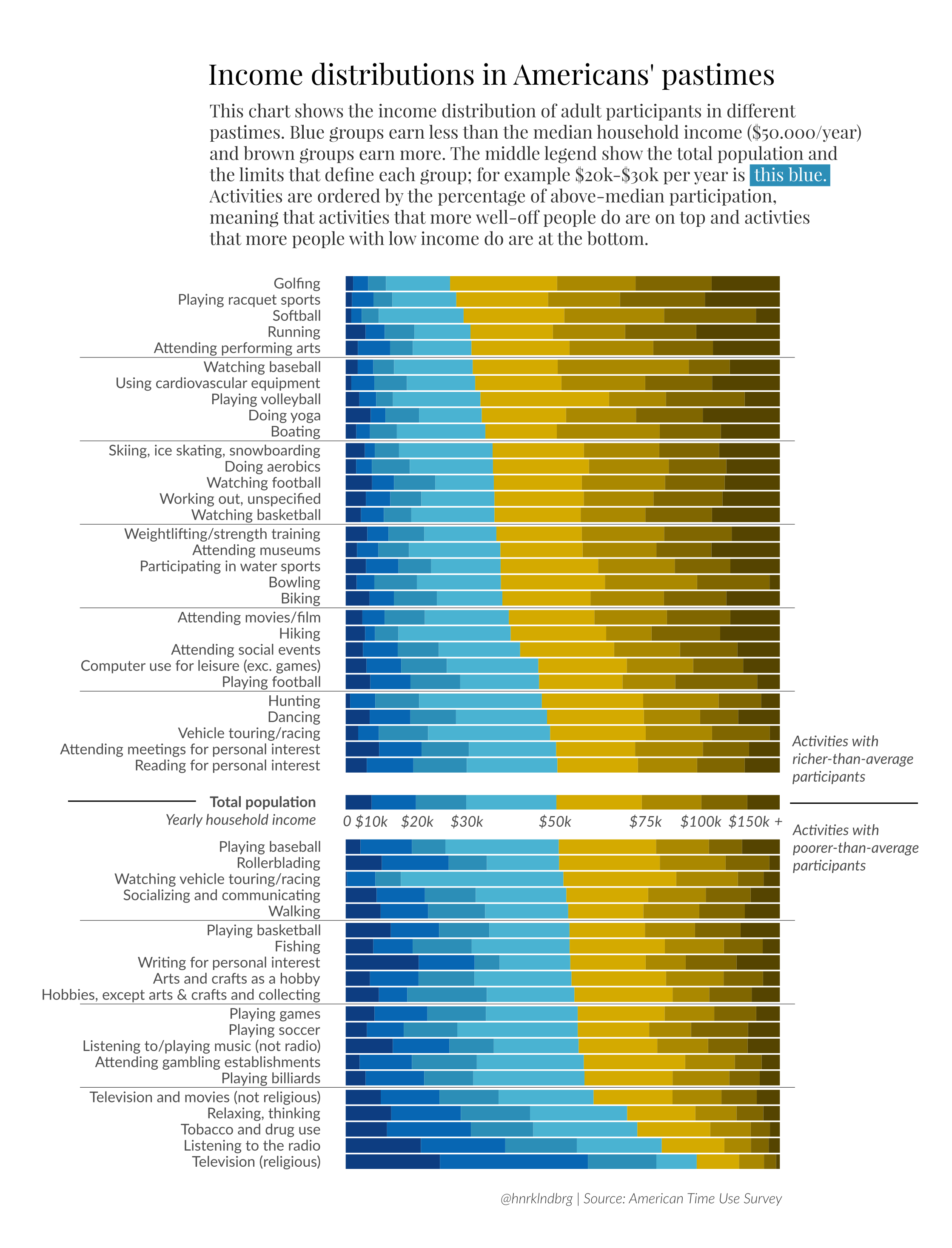
## save the plot above
ggsave(filename = "activity_by_income.png", plot = last_plot(), path = "/cloud/project/atus_survey_analysis/figures/explanatory_figures" )

## Saving 7 x 5 in image

American Time Use Survey Analysis

Rihad Variawa

27/01/2019

Data

Accessing the Data

Loading the Data into R

Importing data

Exploratory Analysis of Child Care Data

Regression Analysis

Exploratory Analysis of Age and Activities

Exploratory Analysis of Income and Activities