Regression discontinuity: banking recovery
K. Richardson
Introduction
After a debt has been legally declared “uncollectable” by a bank, the account is considered to be “charged-off.” But that doesn’t mean the bank simply walks away from the debt. They still want to collect some of the money they are owed. The bank will score the account to assess the expected recovery amount, that is, the expected amount that the bank may be able to receive from the customer in the future (for a fixed time period such as one year). This amount is a function of the probability of the customer paying, the total debt, and other factors that impact the ability and willingness to pay.
The bank has implemented different recovery strategies at different thresholds ($1000, $2000, etc.) where the greater the expected recovery amount, the more effort the bank puts into contacting the customer. For low recovery amounts (Level 0), the bank just adds the customer’s contact information to their automatic dialer and emailing system. For higher recovery strategies, the bank incurs more costs as they leverage human resources in more efforts to contact the customer and obtain payments. Each additional level of recovery strategy requires an additional $50 per customer so that customers in the Recovery Strategy Level 1 cost the company $50 more than those in Level 0. Customers in Level 2 cost $50 more than those in Level 1, etc.
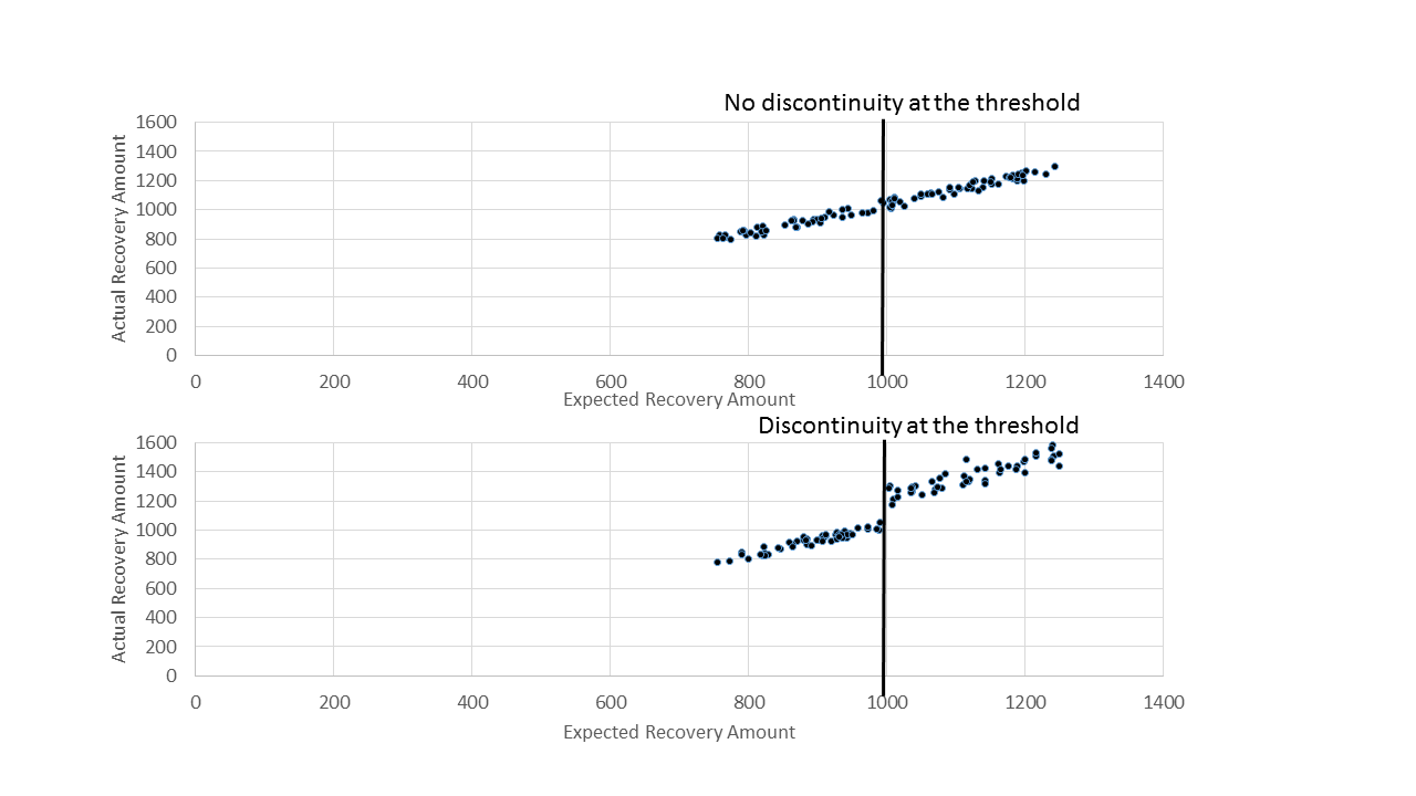
The big question: does the extra amount that is recovered at the higher strategy level exceed the extra $50 in costs? In other words, was there a jump (also called a “discontinuity”) of more than $50 in the amount recovered at the higher strategy level? We’ll find out in this notebook. Click the “Regression discontinuity graph” link below to get a visual representation of discontinuity.
Regression discontinuity graph
First, we’ll load the banking dataset and look at the first few rows of data. This puts us in a good position to understand the dataset itself and begin thinking about how to analyze the data.
# Read in dataset
df <- read_csv("bank_data.csv")
## Parsed with column specification:
## cols(
## id = col_integer(),
## expected_recovery_amount = col_integer(),
## actual_recovery_amount = col_double(),
## recovery_strategy = col_character(),
## age = col_integer(),
## sex = col_character()
## )# Print the first few rows of the DataFrame
head(df)## # A tibble: 6 x 6
## id expected_recovery… actual_recovery_a… recovery_strate… age sex
## <int> <int> <dbl> <chr> <int> <chr>
## 1 2030 194 264. Level 0 Recovery 19 Male
## 2 1150 486 416. Level 0 Recovery 25 Fema…
## 3 380 527 429. Level 0 Recovery 27 Male
## 4 1838 536 297. Level 0 Recovery 25 Male
## 5 1995 541 346. Level 0 Recovery 34 Male
## 6 731 548 521. Level 0 Recovery 35 Male2. Graphical exploratory data analysis
The bank has implemented different recovery strategies at different thresholds ($1000, $2000, $3000 and $5000) where the greater the Expected Recovery Amount, the more effort the bank puts into contacting the customer. Zeroing in on the first transition (between Level 0 and Level 1) means we are focused on the population with Expected Recovery Amounts between $0 and $2000 where the transition between Levels occurred at $1000. We know that the customers in Level 1 (expected recovery amounts between $1001 and $2000) received more attention from the bank and, by definition, they had higher Expected Recovery Amounts than the customers in Level 0 (between $1 and $1000). Here’s a quick summary of the Levels and thresholds again:
Level 0: Expected recovery amounts > $0 and <= $1000 Level 1: Expected recovery amounts > $1000 and <=$2000 The threshold of $1000 separates Level 0 from Level 1
A key question is whether there are other factors besides Expected Recovery Amount that also varied systematically across the $1000 threshold. For example, does the customer age show a jump (discontinuity) at the $1000 threshold or does that age vary smoothly? We can examine this by first making a scatter plot of the age as a function of Expected Recovery Amount for a small window of Expected Recovery Amount, $0 to $2000. This range covers Levels 0 and 1.
# Scatter plot of Age vs. Expected Recovery Amount
ggplot(df, aes(x = expected_recovery_amount, y = age)) + geom_point() + coord_cartesian(xlim = c(0, 2000), ylim = c(0, 60)) + labs(x = "Expected Recovery Amount", y = "Age", title = "Age vs Expected Recovery Amount")
3. Statistical test: age vs. expected recovery amount
We want to convince ourselves that variables such as age and sex are similar above and below the $1000 Expected Recovery Amount threshold. This is important because we want to be able to conclude that differences in the actual recovery amount are due to the higher Recovery Strategy and not due to some other difference like age or sex. The scatter plot of age versus Expected Recovery Amount did not show an obvious jump around $1000. We will be more confident in our conclusions if we do statistical analysis examining the average age of the customers just above and just below the threshold. We can start by exploring the range from $900 to $1100. For determining if there is a difference in the ages just above and just below the threshold, we will use the Kruskal-Wallis test which is a statistical test that makes no distributional assumptions. The test determines whether the population median of two groups are different.
# Compute average age just below and above the threshold
era_900_1100 <- df %>% filter(expected_recovery_amount >= 900 & expected_recovery_amount < 1100)

#convert the recovery strategy variable to a factor
era_900_1100$recovery_strategy <- factor(era_900_1100$recovery_strategy)

#Get the ages for each recovery level
Level_0_Age <- filter(era_900_1100, recovery_strategy == "Level 0 Recovery") %>% pull(age)
Level_1_Age <- filter(era_900_1100, recovery_strategy == "Level 1 Recovery") %>% pull(age)

#Perform Kruskal-Wallis test
kruskal.test(list(Level_0_Age, Level_1_Age))
##
## Kruskal-Wallis rank sum test
##
## data: list(Level_0_Age, Level_1_Age)
## Kruskal-Wallis chi-squared = 3.4572, df = 1, p-value = 0.06298A p-value of 0.06298 is greater than the 0.05 significance level. We can conclude that there is no difference in ages just below and just above the threshold of 1000.
4. Statistical test: sex vs. expected recovery amount
We were able to convince ourselves that there is no major jump in the average customer age just above and just below the $1000 threshold by doing a statistical test as well as exploring it graphically with a scatter plot. We want to also test that the percentage of customers that are male does not jump as well across the $1000 threshold. We can start by exploring the range of $900 to $1100 and later adjust this range. We can examine this question statistically by developing cross-tabs as well as doing chi-square tests of the percentage of customers that are male vs. female.
# Number of customers in each category
cross_tab <- table(era_900_1100$sex, era_900_1100$recovery_strategy)

print(cross_tab)
##
## Level 0 Recovery Level 1 Recovery
## Female 32 39
## Male 57 55# Chi-square test
chisq.test(cross_tab)##
## Pearson's Chi-squared test with Yates' continuity correction
##
## data: cross_tab
## X-squared = 0.37964, df = 1, p-value = 0.5378The Chi-square test gives a p-value of 0.5378 which is not significant. This suggests that sex and recovery strategy are independent. Also, the proportion of males in each recovery strategy are relatively similar.
5. Exploratory graphical analysis: recovery amount
We are now reasonably confident that customers just above and just below the $1000 threshold are, on average, similar in terms of their average age and the percentage that are male. It is now time to focus on the key outcome of interest, the actual recovery amount. A first step in examining the relationship between the actual recovery amount and the expected recovery amount is to develop a scatter plot where we want to focus our attention at the range just below and just above the threshold. Specifically, we will develop a scatter plot of Expected Recovery Amount (X) vs. Actual Recovery Amount (Y) for Expected Recovery Amounts between $900 to $1100. This range covers Levels 0 and 1. A key question is whether or not we see a discontinuity (jump) around the $1000 threshold.
# Scatter plot of Actual Recovery Amount vs. Expected Recovery Amount
ggplot(df, aes(y = actual_recovery_amount, x = expected_recovery_amount)) + geom_point() + labs(x = "Expected Recovery Amount", y = "Actual Recovery Amount", title = "Expected Recovery Amount vs. Actual Recovery Amount") + coord_cartesian(xlim = c(900, 1100), ylim = c(0, 2000))
The scatter plot does not exhibit discontinuity. We observe a generally smooth variation in the actual recovery amount around the $1000 threshold. We can see that level 0 data points have many more than the 3 level 1 data points <= $500 in actual recovery amount. We can also observe several level one points which have actual recovery amount > $1500 while level 0 has none. So we can expect the average actual recovery amount for level 0 to be less than the average actual recovery amount for level 1.
6. Statistical analysis: recovery amount
Just as we did with age, we can perform statistical tests to see if the actual recovery amount has a discontinuity above the $1000 threshold. We are going to do this for two different windows of the expected recovery amount $900 to $1100 and for a narrow range of $950 to $1050 to see if our results are consistent. Again, the statistical test we will use is the Kruskal-Wallis test, a test that makes no assumptions about the distribution of the actual recovery amount. We will first compute the average actual recovery amount for those customers just below and just above the threshold using a range from $900 to $1100. Then we will perform a Kruskal-Wallis test to see if the actual recovery amounts are different just above and just below the threshold. Once we do that, we will repeat these steps for a smaller window of $950 to $1050.
# For the range of $900 to $1100 compute average actual recovery amount just below and above the threshold
Level_0_actual <- filter(era_900_1100, recovery_strategy == "Level 0 Recovery") %>% pull(actual_recovery_amount)
Level_1_actual <- filter(era_900_1100, recovery_strategy == "Level 1 Recovery") %>% pull(actual_recovery_amount)


mean(Level_0_actual)
## [1] 623.017mean(Level_1_actual)## [1] 955.8256# Perform Kruskal-Wallis test
kruskal.test(list(Level_0_actual, Level_1_actual))##
## Kruskal-Wallis rank sum test
##
## data: list(Level_0_actual, Level_1_actual)
## Kruskal-Wallis chi-squared = 65.38, df = 1, p-value = 6.177e-16# Repeat for a smaller range of $950 to $1050
era_950_1050 <- era_900_1100 %>% filter(expected_recovery_amount >= 950 & expected_recovery_amount < 1050)
Level_0_actual_2 <- filter(era_950_1050, recovery_strategy == "Level 0 Recovery") %>% pull(actual_recovery_amount)
Level_1_actual_2 <- filter(era_950_1050, recovery_strategy == "Level 1 Recovery") %>% pull(actual_recovery_amount)
mean(Level_0_actual_2)## [1] 626.1403mean(Level_1_actual_2)## [1] 947.0355kruskal.test(list(Level_0_actual_2, Level_1_actual_2))##
## Kruskal-Wallis rank sum test
##
## data: list(Level_0_actual_2, Level_1_actual_2)
## Kruskal-Wallis chi-squared = 30.246, df = 1, p-value = 3.806e-08For the range of $900 to $1100, the resulting p-value is almost zero which suggests that the medians for the actual recovery amounts just above the threshold and just below the threshold are different.
For the range of $950 to $1050, the resulting p-value is also close to zero which implies that the medians for the actual recovery amounts just above the threshold and just below the threshold are different.
7. Regression modeling: no threshold
We now want to take a regression-based approach to estimate the impact of the program at the $1000 threshold using the data that is just above and just below the threshold. In order to do that, we will build two models. The first model does not have a threshold while the second model will include a threshold. The first model predicts the actual recovery amount (outcome or dependent variable) as a function of the expected recovery amount (input or independent variable). We expect that there will be a strong positive relationship between these two variables. We will examine the adjusted R-squared to see the percent of variance that is explained by the model. In this model, we are not trying to represent the threshold but simply trying to see how the variable used for assigning the customers (expected recovery amount) relates to the outcome variable (actual recovery amount).
# Build linear regression model
model <- lm(actual_recovery_amount ~ expected_recovery_amount, data = era_900_1100)

p <- predict(model, era_900_1100)

# Print out the model summary statistics
summary(model)
##
## Call:
## lm(formula = actual_recovery_amount ~ expected_recovery_amount,
## data = era_900_1100)
##
## Residuals:
## Min 1Q Median 3Q Max
## -544.25 -184.16 -11.49 128.80 1204.50
##
## Coefficients:
## Estimate Std. Error t value Pr(>|t|)
## (Intercept) -1978.7597 347.7409 -5.690 5.02e-08 ***
## expected_recovery_amount 2.7577 0.3453 7.986 1.56e-13 ***
## ---
## Signif. codes: 0 '***' 0.001 '**' 0.01 '*' 0.05 '.' 0.1 ' ' 1
##
## Residual standard error: 263.8 on 181 degrees of freedom
## Multiple R-squared: 0.2606, Adjusted R-squared: 0.2565
## F-statistic: 63.78 on 1 and 181 DF, p-value: 1.563e-138. Regression modeling: adding true threshold
From the first model, we see that the regression coefficient is statistically significant for the expected recovery amount and the adjusted R-squared value was about 0.26. As we saw from the graph, on average the actual recovery amount increases as the expected recovery amount increases. We could add polynomial terms of expected recovery amount (such as the squared value of expected recovery amount) to the model but, for the purposes of this practice, let’s stick with using just the linear term. The second model adds an indicator of the true threshold to the model. If there was no impact of the higher recovery strategy on the actual recovery amount, then we would expect that the relationship between the expected recovery amount and the actual recovery amount would be continuous.
In this case, we know the true threshold is at $1000. We will create an indicator variable (either a 0 or a 1) that represents whether or not the expected recovery amount was greater than $1000. When we add the true threshold to the model, the regression coefficient for the true threshold represents the additional amount recovered due to the higher recovery strategy. That is to say, the regression coefficient for the true threshold measures the size of the discontinuity for customers just above and just below the threshold. If the higher recovery strategy did help recover more money, then the regression coefficient of the true threshold will be greater than zero. If the higher recovery strategy did not help recover more money than the regression coefficient will not be statistically significant.
# Create indicator (0 or 1) for expected recovery amount >= $1000
era_900_1100 <- era_900_1100 %>% mutate(indicator_1000 = ifelse(expected_recovery_amount < 1000, 0, 1))

# Build linear regression model
threshold_model <- lm(actual_recovery_amount ~ expected_recovery_amount + indicator_1000, data = era_900_1100)

#mean confidence interval
confint(threshold_model, level = 0.95)
## 2.5 % 97.5 %
## (Intercept) -1232.4398770 1239.127927
## expected_recovery_amount -0.6498607 1.935827
## indicator_1000 131.5297273 423.739110# Print the model summary
summary(threshold_model)##
## Call:
## lm(formula = actual_recovery_amount ~ expected_recovery_amount +
## indicator_1000, data = era_900_1100)
##
## Residuals:
## Min 1Q Median 3Q Max
## -537.06 -154.69 -34.68 114.29 1108.08
##
## Coefficients:
## Estimate Std. Error t value Pr(>|t|)
## (Intercept) 3.3440 626.2744 0.005 0.995746
## expected_recovery_amount 0.6430 0.6552 0.981 0.327729
## indicator_1000 277.6344 74.0434 3.750 0.000239 ***
## ---
## Signif. codes: 0 '***' 0.001 '**' 0.01 '*' 0.05 '.' 0.1 ' ' 1
##
## Residual standard error: 254.7 on 180 degrees of freedom
## Multiple R-squared: 0.3141, Adjusted R-squared: 0.3065
## F-statistic: 41.22 on 2 and 180 DF, p-value: 1.828e-159. Regression modeling: adjusting the window
The regression coefficient for the true threshold was statistically significant with an estimated impact of around $278 and a 95 percent confidence interval of $132 to $424. This is much larger than the incremental cost of running the higher recovery strategy which was $50 per customer. At this point, we are feeling reasonably confident that the higher recovery strategy is worth the additional costs of the program for customers just above and just below the threshold. Before showing this to our managers, we want to convince ourselves that this result wasn’t due just to us choosing a window of $900 to $1100 for the expected recovery amount. If the higher recovery strategy really had an impact of an extra few hundred dollars, then we should see a similar regression coefficient if we choose a slightly bigger or a slightly smaller window for the expected recovery amount. Let’s repeat this analysis for the window of expected recovery amount from $950 to $1050 to see if we get similar results. The answer? Whether we use a wide window ($900 to $1100) or a narrower window ($950 to $1050), the incremental recovery amount at the higher recovery strategy is much greater than the $50 per customer it costs for the higher recovery strategy. So we can say that the higher recovery strategy is worth the extra $50 per customer that the bank is spending.
# Redefine era_950_1050 so the indicator variable is included
era_950_1050 <- era_950_1050 %>% mutate(indicator_1000 = ifelse(expected_recovery_amount < 1000, 0, 1))

# Build linear regression model
threshold_model_2 <- lm(actual_recovery_amount ~ expected_recovery_amount + indicator_1000, data = era_950_1050)

#mean confidence interval
confint(threshold_model_2)
## 2.5 % 97.5 %
## (Intercept) -3933.298232 3374.249631
## expected_recovery_amount -2.825438 4.663304
## indicator_1000 65.501792 507.565514# Print the model summary
summary(threshold_model_2)##
## Call:
## lm(formula = actual_recovery_amount ~ expected_recovery_amount +
## indicator_1000, data = era_950_1050)
##
## Residuals:
## Min 1Q Median 3Q Max
## -466.32 -161.18 -72.22 102.43 1099.75
##
## Coefficients:
## Estimate Std. Error t value Pr(>|t|)
## (Intercept) -279.5243 1840.7067 -0.152 0.8796
## expected_recovery_amount 0.9189 1.8863 0.487 0.6273
## indicator_1000 286.5337 111.3519 2.573 0.0116 *
## ---
## Signif. codes: 0 '***' 0.001 '**' 0.01 '*' 0.05 '.' 0.1 ' ' 1
##
## Residual standard error: 269.3 on 96 degrees of freedom
## Multiple R-squared: 0.2835, Adjusted R-squared: 0.2685
## F-statistic: 18.99 on 2 and 96 DF, p-value: 1.125e-07For the smaller interval, the regression coefficient for the true threshold was statistically significant (< 0.05) with an estimated impact of around $287 and a 95 percent confidence interval of $66 to $508. This is larger than the incremental cost of running the higher recovery strategy which was $50 per customer.
Conclusion
Whether we use a wide window ($900 to $1100) or a narrower window ($950 to $1050), the incremental recovery amount at the higher recovery strategy is much greater than the $50 per customer it costs for the higher recovery strategy. So we can say that the higher recovery strategy is worth the extra $50 per customer that the bank is spending.