March 13th - March 15th, 2019

Instructors

Alencar Xavier

  • Quantitative Geneticist, Corteva Agrisciences
  • Adjunct professor, Dpt. of Agronomy, Purdue University

Luiz Brito

  • Assistant Professor of Animal Sciences, Purdue University

Hinayah Oliveira

  • Post-doc, Dtp. of Animal Sciences, Purdue University

Katy Rainey

  • Associate Professor, Dpt. of Agronomy, Purdue University

Schedule

  • Module 1: Intro to mixed models
  • Module 2: Fitting mixed models
  • Module 3: Advanced topics
  • Module 4: Signal detection
  • Module 5: Association analysis

Module 1 - Introduction to mixed models

Outline

Part 1: Concepts

  • History of mixed models
  • Mixed models in plant breeding
  • Fixed and random terms
  • Model notation
  • Variance decomposition

Part 2: Applications

  • Selection models
  • Practical examples
  • Variance components
  • Ridges and Kernels

Part 1 - Concepts

History of mixed models

Francis Galton - 1886: Regression and heritability

Ronald Fisher - 1918: Infinitesimal model (P = G + E)

Sewall Wright - 1922: Genetic relationship

Charles Henderson - 1968: BLUP using relationship

Mixed models in plant breeding

Fixed and random terms

Fixed effect

  • Assumed to be invariable (often you cannot recollect the data)
  • Inferences are made upon the parameters
  • Results can not be extrapolated to other datasets
  • Example: Overall mean and environmental effects

Random effects

  • You may not have all the levels available
  • Inference are made on variance components
  • Prior assumption: coefficients are normally distributed
  • Results can not be extrapolated to other datasets
  • Example: Genetic effects

Let's unleash the beast

Model notation

  • Linear model: \(y=Xb+Zu+e\)
  • With variance: \(y \sim N(Xb,ZKZ\sigma^{2}_{u}+I\sigma^{2}_{e})\)

Assuming: \(u \sim N(0,K\sigma^{2}_{u})\) and \(e \sim N(0,I\sigma^{2}_{e})\)

Henderson equation

\[ \left[\begin{array}{rr} X'X & Z'X \\ X'Z & Z'Z+\lambda K^{-1} \end{array}\right] \left[\begin{array}{r} b \\ u \end{array}\right] =\left[\begin{array}{r} X'y \\ Z'y \end{array}\right] \] Summary:

  • We know (data): \(x=\{y,X,Z,K\}\)
  • We want (parameters): \(\theta=\{b,u,\sigma^{2}_{a},\sigma^{2}_{e}\}\)
  • Estimation based on Gaussian likelihood: \(L(x|\theta)\)

Model notation

  • y = vector of observations (n)
  • X = design matrix of fixed effects (n x p)
  • Z = design (or incidence) matrix of random effects (n x q)
  • K = random effect correlation matrix (q x q)
  • u = vector of random effect coefficients (q)
  • b = vector of fixed effect coefficients (p)
  • e = vector of residuals (n)
  • \(\sigma^{2}_{a}\) = marker effect variance (1)
  • \(\sigma^{2}_{u}\) = random effect variance (1)
  • \(\sigma^{2}_{e}\) = residual variance (1)
  • \(\lambda=\sigma^{2}_{e}/\sigma^{2}_{u}\) (Regularization parameters) (1)

Model notation

The mixed model can also be notated as follows

\[y=Wg+e\]

Solved as

\[[W'W+\Sigma] g = [W'y]\]

Where

\(W=[X,Z]\)

\(g=[b,u]\)

\(\Sigma = \left[\begin{array}{rr} 0 & 0 \\ 0 & \lambda K^{-1} \end{array}\right]\)

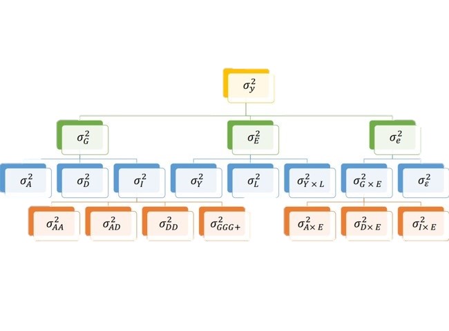
Variance decomposition

Part 2 - Applications

Selection

1 Genetic values

  • BLUPs or BLUEs from replicated trials
  • Captures additive and non-additive genetics together

2 Breeding values

  • Use pedigree information to create \(K\)
  • Captures additive genetics (heritable)
  • Trials not necessarily replicated

3 Genomic Breeding values

  • Genotypic information replaces pedigree
  • Any signal: additivity, dominance and epistasis

Examples

  • Example 1: Balanced data, no kinship
  • Example 2: Balanced data, with kinship
  • Example 3: Unbalanced data, with kinship
  • Example 4: Balanced data, missing individual

Example 1

Data:

##    Env Gen Phe
## 1   E1  G1  47
## 2   E1  G2  51
## 3   E1  G3  46
## 4   E1  G4  58
## 5   E2  G1  52
## 6   E2  G2  46
## 7   E2  G3  52
## 8   E2  G4  54
## 9   E3  G1  53
## 10  E3  G2  48
## 11  E3  G3  58
## 12  E3  G4  52

Model: \(Phenotype = Environment_{(F)} + Genotype_{(R)}\)

Example 1

Design matrix \(W\):

##    EnvE1 EnvE2 EnvE3 GenG1 GenG2 GenG3 GenG4
## 1      1     0     0     1     0     0     0
## 2      1     0     0     0     1     0     0
## 3      1     0     0     0     0     1     0
## 4      1     0     0     0     0     0     1
## 5      0     1     0     1     0     0     0
## 6      0     1     0     0     1     0     0
## 7      0     1     0     0     0     1     0
## 8      0     1     0     0     0     0     1
## 9      0     0     1     1     0     0     0
## 10     0     0     1     0     1     0     0
## 11     0     0     1     0     0     1     0
## 12     0     0     1     0     0     0     1

Example 1

\(W'W\):

##       EnvE1 EnvE2 EnvE3 GenG1 GenG2 GenG3 GenG4
## EnvE1     4     0     0     1     1     1     1
## EnvE2     0     4     0     1     1     1     1
## EnvE3     0     0     4     1     1     1     1
## GenG1     1     1     1     3     0     0     0
## GenG2     1     1     1     0     3     0     0
## GenG3     1     1     1     0     0     3     0
## GenG4     1     1     1     0     0     0     3

Example 1

Left-hand side (\(W'W+\Sigma\)):

##       EnvE1 EnvE2 EnvE3 GenG1 GenG2 GenG3 GenG4
## EnvE1     4     0     0  1.00  1.00  1.00  1.00
## EnvE2     0     4     0  1.00  1.00  1.00  1.00
## EnvE3     0     0     4  1.00  1.00  1.00  1.00
## GenG1     1     1     1  3.17  0.00  0.00  0.00
## GenG2     1     1     1  0.00  3.17  0.00  0.00
## GenG3     1     1     1  0.00  0.00  3.17  0.00
## GenG4     1     1     1  0.00  0.00  0.00  3.17

Assuming independent individuals: \(K=I\)

Regularization: \(\lambda=\sigma^{2}_{e}/\sigma^{2}_{u}=1.64/9.56=0.17\)

Example 1

Right-hand side (\(W'y\)):

##       [,1]
## EnvE1  202
## EnvE2  204
## EnvE3  211
## GenG1  152
## GenG2  145
## GenG3  156
## GenG4  164

Example 1

We can find coefficients through least-square solution

\(g=(LHS)^{-1}(RHS)=(W'W+\Sigma)^{-1}W'y\)

##        [,1]
## EnvE1 50.50
## EnvE2 51.00
## EnvE3 52.75
## GenG1 -0.71
## GenG2 -2.92
## GenG3  0.55
## GenG4  3.08

Shrinkage

\(BLUE=\frac{w'y}{w'w}=\frac{sum}{n}\) = simple average

\(BLUP=\frac{w'y}{w'w+\lambda}=\frac{sum}{n+\lambda}\) = biased average = \(BLUE\times h^2\)

Note:

  • More observations = less shrinkage
  • Higher heritability = less shrinkage: \(\lambda = \frac{h^{2}-1}{h^2}\)

Example 2

If we know the relationship among individuals:

##       GenG1 GenG2 GenG3 GenG4
## GenG1  1.00  0.64  0.23  0.48
## GenG2  0.64  1.00  0.33  0.67
## GenG3  0.23  0.33  1.00  0.31
## GenG4  0.48  0.67  0.31  1.00

Example 2

Then we estimate \(\lambda K^{-1}\)

##       GenG1 GenG2 GenG3 GenG4
## GenG1  0.15 -0.09  0.00 -0.01
## GenG2 -0.09  0.22 -0.02 -0.10
## GenG3  0.00 -0.02  0.10 -0.02
## GenG4 -0.01 -0.10 -0.02  0.17

Regularization: \(\lambda=\sigma^{2}_{e}/\sigma^{2}_{u}=1.64/17.70=0.09\)

Example 2

And the left-hand side becomes

##       EnvE1 EnvE2 EnvE3 GenG1 GenG2 GenG3 GenG4
## EnvE1     4     0     0  1.00  1.00  1.00  1.00
## EnvE2     0     4     0  1.00  1.00  1.00  1.00
## EnvE3     0     0     4  1.00  1.00  1.00  1.00
## GenG1     1     1     1  3.15 -0.09  0.00 -0.01
## GenG2     1     1     1 -0.09  3.22 -0.02 -0.10
## GenG3     1     1     1  0.00 -0.02  3.10 -0.02
## GenG4     1     1     1 -0.01 -0.10 -0.02  3.17

Example 2

We can find coefficients through least-square solution

\(g=(LHS)^{-1}(RHS)=(W'W+\Sigma)^{-1}W'y\)

##        [,1]
## EnvE1 51.05
## EnvE2 51.55
## EnvE3 53.30
## GenG1 -1.32
## GenG2 -3.34
## GenG3  0.03
## GenG4  2.45

Genetic coefficients shrink more: Var(A) < Var(G)

Example 3

What if we have missing data?

##    Env Gen Phe
## 1   E1  G1  47
## 2   E1  G2  51
## 3   E1  G3  NA
## 4   E1  G4  58
## 5   E2  G1  52
## 6   E2  G2  46
## 7   E2  G3  52
## 8   E2  G4  NA
## 9   E3  G1  53
## 10  E3  G2  48
## 11  E3  G3  58
## 12  E3  G4  52

Example 3

Rows of missing points are removed

##    EnvE1 EnvE2 EnvE3 GenG1 GenG2 GenG3 GenG4
## 1      1     0     0     1     0     0     0
## 2      1     0     0     0     1     0     0
## 4      1     0     0     0     0     0     1
## 5      0     1     0     1     0     0     0
## 6      0     1     0     0     1     0     0
## 7      0     1     0     0     0     1     0
## 9      0     0     1     1     0     0     0
## 10     0     0     1     0     1     0     0
## 11     0     0     1     0     0     1     0
## 12     0     0     1     0     0     0     1

Example 3

\(W'W\):

##       EnvE1 EnvE2 EnvE3 GenG1 GenG2 GenG3 GenG4
## EnvE1     3     0     0     1     1     0     1
## EnvE2     0     3     0     1     1     1     0
## EnvE3     0     0     4     1     1     1     1
## GenG1     1     1     1     3     0     0     0
## GenG2     1     1     1     0     3     0     0
## GenG3     0     1     1     0     0     2     0
## GenG4     1     0     1     0     0     0     2

Example 3

Left-hand side (\(W'W+\Sigma\)):

##       EnvE1 EnvE2 EnvE3 GenG1 GenG2 GenG3 GenG4
## EnvE1     3     0     0  1.00  1.00  0.00  1.00
## EnvE2     0     3     0  1.00  1.00  1.00  0.00
## EnvE3     0     0     4  1.00  1.00  1.00  1.00
## GenG1     1     1     1  3.10 -0.06  0.00 -0.01
## GenG2     1     1     1 -0.06  3.15 -0.01 -0.07
## GenG3     0     1     1  0.00 -0.01  2.07 -0.01
## GenG4     1     0     1 -0.01 -0.07 -0.01  2.11

Regularization: \(\lambda=\sigma^{2}_{e}/\sigma^{2}_{u}=1.21/19.61=0.06\)

Example 3

Right-hand side (\(W'y\)):

##       [,1]
## EnvE1  156
## EnvE2  150
## EnvE3  211
## GenG1  152
## GenG2  145
## GenG3  110
## GenG4  110

Example 3

Find coefficients through least-square solution

\(g=(LHS)^{-1}(RHS)=(W'W+\Sigma)^{-1}W'y\)

##        [,1]
## EnvE1 54.14
## EnvE2 51.70
## EnvE3 53.82
## GenG1 -2.56
## GenG2 -4.68
## GenG3  2.15
## GenG4  0.81

Example 4

What if we are missing data from a individual?

##    Env Gen Phe
## 1   E1  G1  NA
## 2   E1  G2  51
## 3   E1  G3  46
## 4   E1  G4  58
## 5   E2  G1  NA
## 6   E2  G2  46
## 7   E2  G3  52
## 8   E2  G4  54
## 9   E3  G1  NA
## 10  E3  G2  48
## 11  E3  G3  58
## 12  E3  G4  52

Example 4

Rows of missing points are removed

##    EnvE1 EnvE2 EnvE3 GenG1 GenG2 GenG3 GenG4
## 2      1     0     0     0     1     0     0
## 3      1     0     0     0     0     1     0
## 4      1     0     0     0     0     0     1
## 6      0     1     0     0     1     0     0
## 7      0     1     0     0     0     1     0
## 8      0     1     0     0     0     0     1
## 10     0     0     1     0     1     0     0
## 11     0     0     1     0     0     1     0
## 12     0     0     1     0     0     0     1

Example 4

\(W'W\):

##       EnvE1 EnvE2 EnvE3 GenG1 GenG2 GenG3 GenG4
## EnvE1     3     0     0     0     1     1     1
## EnvE2     0     3     0     0     1     1     1
## EnvE3     0     0     3     0     1     1     1
## GenG1     0     0     0     0     0     0     0
## GenG2     1     1     1     0     3     0     0
## GenG3     1     1     1     0     0     3     0
## GenG4     1     1     1     0     0     0     3

Example 4

Left-hand side (\(W'W+\Sigma\)):

##       EnvE1 EnvE2 EnvE3 GenG1 GenG2 GenG3 GenG4
## EnvE1     3     0     0  0.00  1.00  1.00  1.00
## EnvE2     0     3     0  0.00  1.00  1.00  1.00
## EnvE3     0     0     3  0.00  1.00  1.00  1.00
## GenG1     0     0     0  0.14 -0.08  0.00 -0.01
## GenG2     1     1     1 -0.08  3.19 -0.02 -0.09
## GenG3     1     1     1  0.00 -0.02  3.09 -0.01
## GenG4     1     1     1 -0.01 -0.09 -0.01  3.15

Regularization: \(\lambda=\sigma^{2}_{e}/\sigma^{2}_{u}=1.79/22.78=0.08\)

Example 4

Right-hand side (\(W'y\)):

##       [,1]
## EnvE1  155
## EnvE2  152
## EnvE3  158
## GenG1    0
## GenG2  145
## GenG3  156
## GenG4  164

Example 4

Find coefficients through least-square solution

\(g=(LHS)^{-1}(RHS)=(W'W+\Sigma)^{-1}W'y\)

##        [,1]
## EnvE1 52.06
## EnvE2 51.06
## EnvE3 53.06
## GenG1 -1.82
## GenG2 -3.48
## GenG3 -0.07
## GenG4  2.38

Variance components

Expectation-Maximization REML (1977)

\(\sigma^{2}_{u} = \frac{u'K^{-1}u}{q-\lambda tr(K^{-1}C^{22})}\) and \(\sigma^{2}_{e} = \frac{e'y}{n-p}\)

Bayesian Gibbs Sampling (1993)

\(\sigma^{2}_{u} = \frac{u'K^{-1}u+S_u\nu_u}{\chi^2(q+\nu_u)}\) and \(\sigma^{2}_{e} = \frac{e'e+S_e\nu_e}{\chi^2(n+\nu_e)}\)

Predicted Residual Error Sum of Squares (PRESS) (2017)

  • \(\lambda = argmin(\sum{e^2_i/(1-h_{ii})^2})\)
  • Where \(H=(I+K\lambda)^{-1}\) and \(e=y-\mu-Hy\)

Ridges and Kernels

Kernel methods:

  • Genetic signal is captured by the relationship matrix \(K\)
  • Random effect coefficients are the breeding values (BV)
  • Efficient to compute BV when \(markers \gg individuals\)
  • Easy use and combine pedigree, markers and interactions

Ridge methods:

  • Genetic signal is captured by the design matrix \(M\)
  • Random effect coefficients are the marker effects
  • Easy way to make predictions of unobserved individuals
  • Enables to visualize where the QTLs are in the genome

Ridges and Kernels

Kernel

\(y=Xb+Zu+e\), \(u\sim N(0,K\sigma^2_u)\)

Ridge

\(y=Xb+Ma+e\), \(a\sim N(0,I\sigma^2_a)\)

Where

  • \(M\) is the genotypic matrix, \(m_{ij}=\{0,1,2\}\)
  • \(K=\alpha MM'\)
  • \(u=Ma\)
  • \(\sigma^2_a=\alpha\sigma^2_u\)

Ridges and Kernels

Kernel model

\[ \left[\begin{array}{rr} X'X & Z'X \\ X'Z & Z'Z+K^{-1}(\sigma^2_e/\sigma^2_u) \end{array}\right] \left[\begin{array}{r} b \\ u \end{array}\right] =\left[\begin{array}{r} X'y \\ Z'y \end{array}\right] \]

Ridge model

\[ \left[\begin{array}{rr} X'X & M'X \\ X'M & M'M+I^{-1}(\sigma^2_e/\sigma^2_a) \end{array}\right] \left[\begin{array}{r} b \\ a \end{array}\right] =\left[\begin{array}{r} X'y \\ M'y \end{array}\right] \]

Both models capture same genetic signal (de los Campos 2015)

Ridges and Kernels

K = tcrossprod(M)/ncol(M)
GBLUP = reml(y=y,K=K); Kernel_GEBV = GBLUP$EBV
RRBLUP = reml(y=y,Z=M); Ridge_GEBV = M%*%RRBLUP$EBV
plot(Kernel_GEBV,Ridge_GEBV, main='Comparing results')

Break

Module 2 - Fitting mixed models

Example 1 - Sorghum

Example 1 - load data

Example dataset from Kevin's agridat package

data(adugna.sorghum, package = 'agridat')
dt = adugna.sorghum
head(dt)
##   gen trial env yield year   loc
## 1 G16    T2 E01   590 2001 Mieso
## 2 G17    T2 E01   554 2001 Mieso
## 3 G18    T2 E01   586 2001 Mieso
## 4 G19    T2 E01   738 2001 Mieso
## 5 G20    T2 E01   489 2001 Mieso
## 6 G21    T2 E01   684 2001 Mieso

Example 1 - Getting design matrix

  • Linear model: \(Pheotype = Env + Gen\)
  • In algebra notation: \(y = Xb + Zu + e\)
y = dt$yield
X = model.matrix(y~env,dt)
Z = model.matrix(y~gen-1,dt) # "-1" means no intercept

Assuming:

  • \(u\sim N(0,I\sigma^2_g)\)
  • \(e\sim N(0,I\sigma^2_e)\)

Example 1 - Visualize X and Z matrices

SEE=function(A,...)image(t(1-A[nrow(A):1,]),axes=F,col=gray.colors(2),...)
par(mfrow=c(1,2),mar=c(1,1,3,1))
SEE(X, main=paste("X matrix (",paste(dim(X),collapse=' x '),")" ))
SEE(Z, main=paste("Z matrix (",paste(dim(Z),collapse=' x '),")" ))

Example 1 - Fit the model

# Using the NAM package (same for rrBLUP, EMMREML, BGLR)
require(NAM, quietly = TRUE)
fit1 = reml(y=y,X=X,Z=Z)
# Alternatively, you can also use formulas with NAM
fit1b = reml(y=dt$yield,X=~dt$env,Z=~dt$gen )
# Using the lme4 package
require(lme4, quietly = TRUE)
fit2 = lmer(yield ~ env + (1|gen), data=dt)

Example 1 - Variance components

fit1$VC[c(1:2)] # same with fit1b$VC
##         Vg       Ve
## 1 189680.4 442075.6
data.frame((summary(fit2))$varcor)$vcov
## [1] 189680.4 442075.6
  • VC can be used to measure broad-sense heritability

\(H=\frac{\sigma^2_g}{\sigma^2_g+\sigma^2_e/n}=\frac{189680.4}{189680.4+442075.6/10.32}=0.82\)

Example 1 - The coefficients

blue1 = fit1$Fixed[,1];  blup1 = fit1$EBV
blue2 = fit2@beta;       blup2 = rowMeans(ranef(fit2)$gen)
par(mfrow=c(1,2));
plot(blue1,blue2,main="BLUE"); plot(blup1,blup2,main="BLUP")

Example 1 - DIY BLUPs

iK = diag(ncol(Z))
Lambda = 442075.6/189680.4
W = cbind(X,Z)
Sigma = as.matrix(Matrix::bdiag(diag(0,ncol(X)),iK*Lambda))
LHS = crossprod(W) + Sigma
RHS = crossprod(W,y)
g = solve(LHS,RHS)
my_blue = g[ c(1:ncol(X))]
my_blup = g[-c(1:ncol(X))]

Example 1 - DIY BLUPs

par(mfrow=c(1,2))
plot(my_blue,blue1,main="BLUE")
plot(my_blup,blup1,main="BLUP")

Example 1 - DIY Variance components

\(\sigma^{2}_{e} = \frac{e'y}{n-p}\) and \(\sigma^{2}_{u} = \frac{u'K^{-1}u+tr(K^{-1}C^{22}\sigma^{2}_{e})}{q}\)

e = y - X %*% my_blue - Z %*% my_blup
Ve = c(y%*%e)/(length(y)-ncol(X))
Ve
## [1] 442075.6
trKC22 = sum(diag(iK%*%(solve(LHS)[-c(1:ncol(X)),-c(1:ncol(X))])))
Vg = Vg = c(t(my_blup)%*%iK%*%my_blup+trKC22*Ve)/ncol(Z)
Vg
## [1] 189680.4

Starting from bad variance components

Ve = Vg = 1
for(i in 1:25){
  Lambda = Ve/Vg; 
  Sigma = as.matrix(Matrix::bdiag(diag(0,ncol(X)),iK*Lambda))
  LHS = crossprod(W) + Sigma; RHS = crossprod(W,y); g = solve(LHS,RHS)
  my_blue = g[ c(1:ncol(X))]; my_blup = g[-c(1:ncol(X))]
  e = y - X%*%my_blue - Z%*%my_blup; Ve = c(y%*%e)/(length(y)-ncol(X))
  trKC22 = sum(diag(iK%*%(solve(LHS)[(ncol(X)+1):(ncol(W)),(ncol(X)+1):(ncol(W))])))
  Vg = c(t(my_blup)%*%iK%*%my_blup+trKC22*Ve)/ncol(Z)
  if(!i%%5){cat('It',i,'VC:  Vg =',Vg,'and Ve =',Ve,'\n')}}
## It 5 VC:  Vg = 191751.1 and Ve = 441110.7 
## It 10 VC:  Vg = 189728.4 and Ve = 442053.2 
## It 15 VC:  Vg = 189681.5 and Ve = 442075.1 
## It 20 VC:  Vg = 189680.4 and Ve = 442075.6 
## It 25 VC:  Vg = 189680.4 and Ve = 442075.6

Example 2 - Barley

Example 2 - load data

Another example dataset from Kevin's agridat package

data(steptoe.morex.pheno,package='agridat')
dt = steptoe.morex.pheno
head(dt)
##       gen   env amylase diapow hddate lodging malt height protein  yield
## 1 Steptoe  MN92    22.7     46  149.5      NA 73.6   84.5    10.5 5.5315
## 2 Steptoe MTi92    30.1     72  178.0      10 76.5     NA    11.2 8.6403
## 3 Steptoe MTd92    26.7     78  165.0      15 74.5   75.5    13.4 5.8990
## 4 Steptoe  ID91    26.2     74  179.0      NA 74.1  111.0    12.1 8.6290
## 5 Steptoe  OR91    19.6     62  191.0      NA 71.5   90.0    11.7 5.3440
## 6 Steptoe  WA91    23.6     54  181.0      NA 73.8  112.0    10.0 6.2700

Example 2 - Getting design matrix

  • Linear model: \(Phe=Env+Gen\)

  • In algebra notation: \(y=Xb+Zu+e\)

X = model.matrix(~env,dt)
Z = model.matrix(~gen-1,dt) # "-1" means no intercept
y = dt$yield

Example 2 - Fit the model

# Fit
fit0 = reml(y=y,X=X,Z=Z)
# BLUE and BLUP
blue0 = fit0$Fixed[,1]
blup0 = fit0$EBV
# Get VC
fit0$VC[c(1:2)]
##          Vg        Ve
## 1 0.1320092 0.6379967

Example 2 - DIY BLUPs

iK = diag(ncol(Z))
Lambda = 0.637997/0.132009
W = cbind(X,Z)
Sigma = as.matrix(Matrix::bdiag(diag(0,ncol(X)),iK*Lambda))
LHS = crossprod(W) + Sigma
RHS = crossprod(W,y)
g = solve(LHS,RHS)
my_blue = g[ c(1:ncol(X))]
my_blup = g[-c(1:ncol(X))]

Example 2 - DIY BLUPs

par(mfrow=c(1,2))
plot(my_blue,blue0,main="BLUE")
plot(my_blup,blup0,main="BLUP")

Example 2 - Check variance components

\(\sigma^{2}_{e} = \frac{e'y}{n-p}\) and \(\sigma^{2}_{u} = \frac{u'K^{-1}u+tr(K^{-1}C^{22}\sigma^{2}_{e})}{q}\)

e = y - X %*% my_blue - Z %*% my_blup
Ve = c(y%*%e)/(length(y)-ncol(X))
Ve
## [1] 0.6379967
trKC22 = sum(diag(iK%*%(solve(LHS)[-c(1:ncol(X)),-c(1:ncol(X))])))
Vg = c(t(my_blup)%*%iK%*%my_blup+trKC22*Ve)/ncol(Z)
Vg
## [1] 0.1320091

Starting from bad variance components

Ve = Vg = 1
for(i in 1:25){
  Lambda = Ve/Vg; 
  Sigma = as.matrix(Matrix::bdiag(diag(0,ncol(X)),iK*Lambda))
  LHS = crossprod(W) + Sigma; RHS = crossprod(W,y); g = solve(LHS,RHS)
  my_blue = g[ c(1:ncol(X))]; my_blup = g[-c(1:ncol(X))]
  e = y - X%*%my_blue - Z%*%my_blup; Ve = c(y%*%e)/(length(y)-ncol(X))
  trKC22 = sum(diag(iK%*%(solve(LHS)[(ncol(X)+1):(ncol(W)),(ncol(X)+1):(ncol(W))])))
  Vg = c(t(my_blup)%*%iK%*%my_blup+trKC22*Ve)/ncol(Z)
  if(!i%%5){cat('It',i,'VC:  Vg =',Vg,'and Ve =',Ve,'\n')}}
## It 5 VC:  Vg = 0.1336139 and Ve = 0.6370751 
## It 10 VC:  Vg = 0.1320386 and Ve = 0.6379797 
## It 15 VC:  Vg = 0.1320097 and Ve = 0.6379964 
## It 20 VC:  Vg = 0.1320092 and Ve = 0.6379967 
## It 25 VC:  Vg = 0.1320092 and Ve = 0.6379967

Example 3 - Barley GEBV

Using genomic information!

data(steptoe.morex.geno,package='agridat')
gen = do.call("cbind",lapply(steptoe.morex.geno$geno,function(x) x$data))
gen = rbind(0,2,gen)
rownames(gen) = c('Morex','Steptoe',as.character(steptoe.morex.geno$pheno$gen))
rownames(gen)[10] = "SM8"
gen = gen[gsub('gen','',colnames(Z)),]
K = GRM(IMP(gen),T)

Example 3 - Fit the model

# Fit model
fit0 = reml(y=y,X=X,Z=Z,K=K)
# BLUE and BLUP
blue0 = fit0$Fixed[,1]
gebv0 = fit0$EBV
# Get VC
fit0$VC[c(1:2)]
##         Vg        Ve
## 1 1.027988 0.6575786

Example 3 - DIY BLUPs

diag(K) = diag(K)+1e-08; iK = solve(K)
Lambda = 0.6575/1.0280
W = cbind(X,Z)
Sigma = as.matrix(Matrix::bdiag(diag(0,ncol(X)),iK*Lambda))
LHS = crossprod(W) + Sigma
RHS = crossprod(W,y)
g = solve(LHS,RHS)
my_blue = g[ c(1:ncol(X))]
my_gebv = g[-c(1:ncol(X))]

Example 3 - DIY BLUPs

par(mfrow=c(1,2))
plot(my_blue,blue0,main="BLUE")
plot(my_gebv,gebv0,main="GEBV")

Example 3 - Check variance components

\(\sigma^{2}_{e} = \frac{e'y}{n-p}\) and \(\sigma^{2}_{u} = \frac{u'K^{-1}u+tr(K^{-1}C^{22}\sigma^{2}_{e})}{q}\)

e = y - X %*% my_blue - Z %*% my_blup
Ve = c(y%*%e)/(length(y)-ncol(X))
Ve
## [1] 0.6379967
trKC22 = sum(diag(iK%*%(solve(LHS)[(ncol(X)+1):(ncol(W)),(ncol(X)+1):(ncol(W))])))
Vg = c(t(my_blup)%*%iK%*%my_blup+trKC22*Ve)/ncol(Z)
Vg
## [1] 14.12085

Example 4 - Soybeans

snp-BLUP

data(tpod,package='NAM')
X = matrix(1,length(y),1)
Z = gen
dim(Z)
## [1] 196 376

Example 4 - Fit the model

# Fit using the lme4 package
fit0 = reml(y=y,X=X,Z=Z) # same as reml(y=y,Z=gen) 
marker_values = fit0$EBV
gebv0 = c(gen %*% marker_values)
# Marker effects
plot(marker_values,pch=16, xlab='SNP')

Example 4 - DIY BLUPs

iK = diag(ncol(Z))
Lambda = fit0$VC[2] / fit0$VC[1]
W = cbind(X,Z)
Sigma = diag( c(0,rep(Lambda,ncol(Z))) )
LHS = crossprod(W) + Sigma
RHS = crossprod(W,y)
g = solve(LHS,RHS)
my_mu = g[ c(1:ncol(X))]
my_marker_values = g[-c(1:ncol(X))]
my_gebv = c(gen %*% my_marker_values) # GEBVs from RR

Example 4 - DIY BLUPs

par(mfrow=c(1,2))
plot(my_marker_values, marker_values, main="Markers")
plot(my_gebv, gebv0, main="GEBV")

Example 4 - Heritability from RR

fit0$VC
##             Vg         Ve           h2
## 1 1.659819e-05 0.03167014 0.0005238214
Scale=sum(apply(gen,2,var)); Va=fit0$VC[1]*Scale;  Ve=fit0$VC[2]
round((Va/(Va+Ve)),2)
##     Vg
## 1 0.16
K = tcrossprod(apply(gen,2,function(x) x-mean(X)))
K = K/mean(diag(K)); round(reml(y,K=K)$VC,2)
##     Vg   Ve   h2
## 1 0.01 0.03 0.16

Estimate VC from bad starters

W = cbind(X,Z); iK = diag(ncol(Z))
Ve = Vg = 1 # Bad starting values
for(i in 1:100){ # Check the VC convergence after few iterations
  Lambda = Ve/Vg; 
  Sigma = as.matrix(Matrix::bdiag(diag(0,ncol(X)),iK*Lambda))
  LHS = crossprod(W) + Sigma; RHS = crossprod(W,y); g = solve(LHS,RHS)
  my_blue = g[ c(1:ncol(X))]; my_blup = g[-c(1:ncol(X))]
  e = y - X%*%my_blue - Z%*%my_blup; Ve = c(y%*%e)/(length(y)-ncol(X))
  trKC22 = sum(diag(iK%*%(solve(LHS)[(ncol(X)+1):(ncol(W)),(ncol(X)+1):(ncol(W))])))
  Vg = c(t(my_blup)%*%iK%*%my_blup+trKC22*Ve)/ncol(Z)
  if(!i%%25){cat('It',i,'VC:  Vg =',Vg,'and Ve =',Ve,'\n')}}
## It 25 VC:  Vg = 0.0002960602 and Ve = 0.01801226 
## It 50 VC:  Vg = 7.428217e-05 and Ve = 0.02531553 
## It 75 VC:  Vg = 4.000965e-05 and Ve = 0.02818575 
## It 100 VC:  Vg = 2.887763e-05 and Ve = 0.02956763

Break

Module 3 - Advanced topics

Outline

  • Multivariate models
  • Bayesian methods
  • Machine learning
  • G x E interactions

Multivariate models

Multivariate models

Mixed models also enable us to evaluate multiple traits:

  • More accurate parameters: BV and variance components
  • Information: Inform how traits relate to each other
  • Constrains: May increase computation time considerably

It preserves the same formulation

\[y = Xb+Zu+e\] However, we now stack the traits together:

\(y=\{y_1,y_2,...,y_k\}\), \(X=\{X_1, X_2, ... , X_k\}'\), \(b=\{b_1,b_2,...,b_k\}\), \(Z=\{Z_1, Z_2, ... , Z_k\}'\), \(u=\{u_1,u_2,...,u_k\}\), \(e=\{e_1,e_2,...,e_k\}\).

Multivariate models

The multivariate variance looks nice at first \[ Var(y) = Var(u) + Var(e) \]

But can get ugly with a closer look:

\[ Var(u) = Z ( G \otimes \Sigma_a ) Z' = \left[\begin{array}{rr} Z_1 G Z_1'\sigma^2_{a_1} & Z_1 G Z_2'\sigma_{a_{12}} \\ Z_2 G Z_1' \sigma_{a_{21}} & Z_2 G Z_2'\sigma^2_{a_2} \end{array}\right] \]

and

\[ Var(e) = R \otimes \Sigma_e = \left[\begin{array}{rr} R\sigma^2_{e_1} & R\sigma_{e_1e_2} \\ R\sigma_{e_2e_1} & R\sigma^2_{e_2} \end{array}\right] \]

Multivariate models

You can still think the multivariate mixed model as

\[y=Wg+e\]

Where

\[ y = \left[\begin{array}{rr} y_1 \\ y_2 \end{array}\right], W = \left[\begin{array}{rr} X_1 & 0 & Z_1 & 0 \\ 0 & X_2 & 0 & Z_2 \\ \end{array}\right], g = \left[\begin{array}{rr} b_1 \\ b_2 \\ u_1 \\ u_2 \end{array}\right], e = \left[\begin{array}{rr} e_1 \\ e_2 \end{array}\right] \]

Multivariate models

Left-hand side (\(W'R^{-1}W+\Sigma\)) \[ \left[\begin{array}{rr} X_1'X_1\Sigma^{-1}_{e_{11}} & X_1'X_2\Sigma^{-1}_{e_{12}} & X_1'Z_1\Sigma^{-1}_{e_{11}} & X_1'Z_2\Sigma^{-1}_{e_{12}}\\ X_2'X_1\Sigma^{-1}_{e_{12}} & X_2'X_2\Sigma^{-1}_{e_{22}} & X_2'Z_1\Sigma^{-1}_{e_{12}} & X_2'Z_2\Sigma^{-1}_{e_{22}}\\ Z_1'X_1\Sigma^{-1}_{e_{11}} & Z_1'X_2\Sigma^{-1}_{e_{12}} & G^{-1}\Sigma^{-1}_{a_{11}} + Z_1'Z_1\Sigma^{-1}_{e_{11}} & G^{-1}\Sigma^{-1}_{a_{12}} + Z_1'Z_2\Sigma^{-1}_{e_{12}}\\ Z_2'X_1\Sigma^{-1}_{e_{12}} & Z_2'X_2\Sigma^{-1}_{e_{22}} & G^{-1}\Sigma^{-1}_{a_{11}} + Z_2'Z_1\Sigma^{-1}_{e_{12}} & G^{-1}\Sigma^{-1}_{a_{22}} + Z_2'Z_2\Sigma^{-1}_{e_{22}}\\ \end{array}\right] \] Right-hand side (\(W'R^{-1}y\)) \[ \left[\begin{array}{rr} X_1'(y_1\Sigma^{-1}_{e_1}+y_2\Sigma^{-1}_{e_12}) \\ X_2'(y_1\Sigma^{-1}_{e_22}+y_2\Sigma^{-1}_{e_12}) \\ Z_1'(y_1\Sigma^{-1}_{e_12}+y_2\Sigma^{-1}_{e_1}) \\ Z_2'(y_1\Sigma^{-1}_{e_12}+y_2\Sigma^{-1}_{e_12}) \\ \end{array}\right] \]

Multivariate models

data(wheat, package = 'BGLR')
G = NAM::GRM(wheat.X);
Y = wheat.Y; colnames(Y) = c('E1','E2','E3','E4')
mmm = NAM::reml( y = Y, K = G )
knitr::kable( round(mmm$VC$GenCor,2) )
E1 E2 E3 E4
E1 1.00 -0.25 -0.22 -0.50
E2 -0.25 1.00 0.96 0.55
E3 -0.22 0.96 1.00 0.72
E4 -0.50 0.55 0.72 1.00

Multivariate models

mmm$VC$Vg
##            E1         E2         E3         E4
## E1  0.6277835 -0.1446924 -0.1102175 -0.2743640
## E2 -0.1446924  0.5440731  0.4419945  0.2822577
## E3 -0.1102175  0.4419945  0.3919626  0.3130735
## E4 -0.2743640  0.2822577  0.3130735  0.4828705
mmm$VC$Ve
##             E1         E2         E3         E4
## E1  0.53504246 0.08247812 -0.1159118 0.06882868
## E2  0.08247812 0.56214755  0.2973841 0.15795801
## E3 -0.11591175 0.29738408  0.6714234 0.11086214
## E4  0.06882868 0.15795801  0.1108621 0.59405228

Multivariate models

  • Selection indeces, co-heritability, indirect response to selection
  • Study residual and additive genetic association among traits
biplot(princomp(mmm$VC$GenCor,cor=T),xlim=c(-.4,.4),ylim=c(-.11,.11))

Multivariate models

When do additional traits contribute?

# Fit E4, predict E2
fit_E4=bWGR::mrr(matrix(Y[,4]),wheat.X); cor(fit_E4$hat[,1],Y[,2])
## [1] 0.3988844
# Fit E4 and E1, E4 predict E2
fit_E4E1=bWGR::mrr(Y[,c(1,4)],wheat.X); cor(fit_E4E1$hat[,2],Y[,2])
## [1] 0.3931193
# Fit E4 and E3, E4 predict E2
fit_E4E3=bWGR::mrr(Y[,3:4],wheat.X); cor(fit_E4E3$hat[,2], Y[,2])
## [1] 0.5279279

Bayesian methods

Bayesian methods

The general framework on a hierarchical Bayesian model follows:

\[p(\theta|x)\propto p(x|\theta) p(\theta)\]

Where:

  • Posterior probability: \(p(\theta|x)\)
  • Likelihood: \(p(x|\theta)\)
  • Prior probability: \(p(\theta)\)

Bayesian methods

For the model:

\[y=Xb+Zu+e, \space\space\space u\sim N(0,K\sigma^2_a), \space e \sim N(0,I\sigma^2_e)\]

  • Data (\(x=\{y,X,Z,K\}\))
  • Parameters (\(\theta=\{b,u,\sigma^2_a,\sigma^2_e\}\))

Probabilistic model:

\[p(b,u,\sigma^2_a,\sigma^2_e|y,X,Z,K) \propto N(y,X,Z,K|b,u,\sigma^2_a,\sigma^2_e) \times \space\space\space\space\space\space\space\space\space\space \space\space\space\space\space\space\space\space\space\space\space\space \space\space\space\space\space\space\space\space\space\space\space\space\space\space \space\space\space\space\space\space\space\space\space\space\space\space \space\space\space\space\space\space\space\space\space\space\space\space\space\space\space\space \space\space\space\space\space\space \\ N(b, u|\sigma^2_a,\sigma^2_e) \times \chi^{-2}(\sigma^2_a,\sigma^2_e|S_a,S_e,\nu_a,\nu_e)\]

Bayesian methods

REML: the priors \((S_a,S_e,\nu_a,\nu_e)\) are estimated from data.

Hierarchical Bayes: You provide priors. Here is how:

\[\sigma^2_a=\frac {u'K^{-1}u+S_a\nu_a} {\chi^2(q+\nu_a)}\]

sigma2a=(t(u)%*%iK%*%u+Sa*dfa)/rchisq(df=ncol(Z)+dfa,n=1)

\[\sigma^2_e=\frac {e'e+S_e\nu_e} {\chi^2(n+\nu_e)}\]

sigma2e=(t(e)%*%e+Se*dfe)/rchisq(df=length(y)+dfe,n=1)

Bayesian methods

What does it mean for you? If your "prior knowledge" tells you that a given trait has approximately \(h^2=0.5\) (nothing unreasonable). In which case, half of the phenotypic variance is due to genetics, and the other half is due to error. Your prior shape is:

\[S_a = S_e= \sigma^2_y\times0.5\]

We usually assign small a prior degrees of freeds. Samething like four or five prior degrees of freedom. That means that assuming \(\nu_0=5\), you are yielding to your model 5 data points that support heritability 0.5

\[\nu_a=\nu_e=5\]

Example of prior influence: In a dataset with 300 data points, 1.6% of the variance components information comes from prior (5/305), and 98.4% comes from data (300/305).

Bayesian methods

For whole-genome regression models

\[y=\mu+Ma+e, \space\space\space a\sim N(0,I\sigma^2_b), \space e\sim N(0,I\sigma^2_e)\]

We scale the prior genetic variance based on allele frequencies

\[ S_b = \frac{\sigma^2_y\times0.5}{2 \sum{p_j(1-p_j)} }\]

Two common settings:

  • All markers, one random effect: Bayesian ridge regression
  • Each markers as a random effect: BayesA

Machine learning methods

  • Parametric methods for prediction: L1-L2
  • Semi-parametric methods for prediction: Kernels
  • Non-parametric methods for prediction: Trees and nets

Machine learning methods

L1-L2 machines include all mixed and Bayesian models we have seen so far. The basic framework is driven by a single (random) term model:

\[y=Xb+e\]

The univariate soltion indicates how the model is solved. A model without regularization yields the least square (LS) solution. If we regularize by deflating the nominator, we get the L1 regularization (LASSO). If we regularize by inflating the denominator, we get the L2 regularization (Ridge). For any combination of both, we get a elastic-net (EN). Thus:

\[b_{LS}=\frac{x'y}{x'x}, \space\space b_{Lasso}=\frac{x'y-\lambda}{x'x}, \space\space b_{Ridge}=\frac{x'y}{x'x+\lambda}, \space\space b_{EN}=\frac{x'y-\lambda_1}{x'x+\lambda_2}\]

Whereas the Bayesian and mixed model framework resolves the regularization as \(\lambda=\sigma^2_e/\sigma^2_b\), ML methods search for \(\lambda\) through (k-fold) cross-validation.

Machine learning methods

Common loss functions in L1-L2 machines

  • LS (no prior, no shrinkage): \(argmin( \sum{e_i^2} )\)
  • L1 (Laplace prior with variable selection): \(argmin( \sum{e_i^2} + \lambda\sum{|b_j|} )\)
  • L2 (Gaussian prior, unique solution): \(argmin( \sum{e_i^2} + \lambda\sum{b^2_j} )\)

Other losses that are less popular

  • Least absolute: \(argmin( \sum{|e_i|} )\) based on \(b_{LA}=\frac{ n MD(x\times y)}{x'x}\)
  • \(\epsilon\)-loss: \(argmin(\sum{e_i^2, |e_i|>\epsilon})\) - used in support vector machines

Machine learning methods

Cross-validations to search for best value of lambda

lasso = glmnet::cv.glmnet(x=wheat.X,y=rowMeans(Y),alpha=1);
ridge = glmnet::cv.glmnet(x=wheat.X,y=rowMeans(Y),alpha=0);
par(mfrow=c(1,2)); plot(ridge); plot(lasso)

Machine learning methods

Re-fit the model using this best value

lasso = glmnet::glmnet(x=wheat.X,y=rowMeans(Y),lambda=lasso$lambda.min,alpha=1)
ridge = glmnet::glmnet(x=wheat.X,y=rowMeans(Y),lambda=ridge$lambda.min,alpha=0)
par(mfrow=c(1,2)); plot(lasso$beta,main='LASSO'); plot(ridge$beta,main='RIDGE');

Machine learning methods

Of course, the losses presented above are not limited to the application of prediction and classification. Below, we see an example of deploying LASSO for a graphical model (Markov Random Field): How the traits of the multivariate model relate in terms of additive genetics:

ADJ=huge::huge(mmm$VC$GenCor,.3,method='glasso',verbose=F)$path[[1]]
plot(igraph::graph.adjacency(adjmatrix=ADJ),vertex.label.cex=3)

Machine learning methods

Reproducing kernel Hilbert Spaces (RKHS), is a generalization of a GBLUP… Most commonly instead of using the linear kernel (\(ZZ'\alpha\)), RKHS commonly uses one or more Gaussian or exponential kernels:

\[K=\exp(-\theta D^2)\]

Where \(D^2\) is the squared Euclidean distance, and \(\theta\) is a bandwidth:

  • Single kernel: \(1/mean(D^2)\)
  • Three kernels: \(\theta\)={5/q, 1/q, 0.2/q}, where q=quantile(D2,0.05)

Machine learning methods

We can use REML, PRESS (=cross-validation) or Bayesian approach to solve RKHS

# Make the kernel
D2 = as.matrix(dist(wheat.X)^2)
K = exp(-D2/mean(D2))
# Below we are going to calibrate models on Env 2 and predict Env 3
rkhs_press = NAM::press(y=Y[,2],K=K)$hat
rkhs_reml = NAM::reml(y=Y[,2],K=K)$EBV
rkhs_bgs = NAM::gibbs(y=Y[,2],iK=solve(K))$Fit.mean
## 
  |                                                                       
  |                                                                 |   0%
  |                                                                       
  |                                                                 |   1%
  |                                                                       
  |=                                                                |   1%
  |                                                                       
  |=                                                                |   2%
  |                                                                       
  |==                                                               |   2%
  |                                                                       
  |==                                                               |   3%
  |                                                                       
  |==                                                               |   4%
  |                                                                       
  |===                                                              |   4%
  |                                                                       
  |===                                                              |   5%
  |                                                                       
  |====                                                             |   5%
  |                                                                       
  |====                                                             |   6%
  |                                                                       
  |====                                                             |   7%
  |                                                                       
  |=====                                                            |   7%
  |                                                                       
  |=====                                                            |   8%
  |                                                                       
  |======                                                           |   8%
  |                                                                       
  |======                                                           |   9%
  |                                                                       
  |======                                                           |  10%
  |                                                                       
  |=======                                                          |  10%
  |                                                                       
  |=======                                                          |  11%
  |                                                                       
  |=======                                                          |  12%
  |                                                                       
  |========                                                         |  12%
  |                                                                       
  |========                                                         |  13%
  |                                                                       
  |=========                                                        |  13%
  |                                                                       
  |=========                                                        |  14%
  |                                                                       
  |=========                                                        |  15%
  |                                                                       
  |==========                                                       |  15%
  |                                                                       
  |==========                                                       |  16%
  |                                                                       
  |===========                                                      |  16%
  |                                                                       
  |===========                                                      |  17%
  |                                                                       
  |===========                                                      |  18%
  |                                                                       
  |============                                                     |  18%
  |                                                                       
  |============                                                     |  19%
  |                                                                       
  |=============                                                    |  19%
  |                                                                       
  |=============                                                    |  20%
  |                                                                       
  |=============                                                    |  21%
  |                                                                       
  |==============                                                   |  21%
  |                                                                       
  |==============                                                   |  22%
  |                                                                       
  |===============                                                  |  22%
  |                                                                       
  |===============                                                  |  23%
  |                                                                       
  |===============                                                  |  24%
  |                                                                       
  |================                                                 |  24%
  |                                                                       
  |================                                                 |  25%
  |                                                                       
  |=================                                                |  25%
  |                                                                       
  |=================                                                |  26%
  |                                                                       
  |=================                                                |  27%
  |                                                                       
  |==================                                               |  27%
  |                                                                       
  |==================                                               |  28%
  |                                                                       
  |===================                                              |  28%
  |                                                                       
  |===================                                              |  29%
  |                                                                       
  |===================                                              |  30%
  |                                                                       
  |====================                                             |  30%
  |                                                                       
  |====================                                             |  31%
  |                                                                       
  |====================                                             |  32%
  |                                                                       
  |=====================                                            |  32%
  |                                                                       
  |=====================                                            |  33%
  |                                                                       
  |======================                                           |  33%
  |                                                                       
  |======================                                           |  34%
  |                                                                       
  |======================                                           |  35%
  |                                                                       
  |=======================                                          |  35%
  |                                                                       
  |=======================                                          |  36%
  |                                                                       
  |========================                                         |  36%
  |                                                                       
  |========================                                         |  37%
  |                                                                       
  |========================                                         |  38%
  |                                                                       
  |=========================                                        |  38%
  |                                                                       
  |=========================                                        |  39%
  |                                                                       
  |==========================                                       |  39%
  |                                                                       
  |==========================                                       |  40%
  |                                                                       
  |==========================                                       |  41%
  |                                                                       
  |===========================                                      |  41%
  |                                                                       
  |===========================                                      |  42%
  |                                                                       
  |============================                                     |  42%
  |                                                                       
  |============================                                     |  43%
  |                                                                       
  |============================                                     |  44%
  |                                                                       
  |=============================                                    |  44%
  |                                                                       
  |=============================                                    |  45%
  |                                                                       
  |==============================                                   |  45%
  |                                                                       
  |==============================                                   |  46%
  |                                                                       
  |==============================                                   |  47%
  |                                                                       
  |===============================                                  |  47%
  |                                                                       
  |===============================                                  |  48%
  |                                                                       
  |================================                                 |  48%
  |                                                                       
  |================================                                 |  49%
  |                                                                       
  |================================                                 |  50%
  |                                                                       
  |=================================                                |  50%
  |                                                                       
  |=================================                                |  51%
  |                                                                       
  |=================================                                |  52%
  |                                                                       
  |==================================                               |  52%
  |                                                                       
  |==================================                               |  53%
  |                                                                       
  |===================================                              |  53%
  |                                                                       
  |===================================                              |  54%
  |                                                                       
  |===================================                              |  55%
  |                                                                       
  |====================================                             |  55%
  |                                                                       
  |====================================                             |  56%
  |                                                                       
  |=====================================                            |  56%
  |                                                                       
  |=====================================                            |  57%
  |                                                                       
  |=====================================                            |  58%
  |                                                                       
  |======================================                           |  58%
  |                                                                       
  |======================================                           |  59%
  |                                                                       
  |=======================================                          |  59%
  |                                                                       
  |=======================================                          |  60%
  |                                                                       
  |=======================================                          |  61%
  |                                                                       
  |========================================                         |  61%
  |                                                                       
  |========================================                         |  62%
  |                                                                       
  |=========================================                        |  62%
  |                                                                       
  |=========================================                        |  63%
  |                                                                       
  |=========================================                        |  64%
  |                                                                       
  |==========================================                       |  64%
  |                                                                       
  |==========================================                       |  65%
  |                                                                       
  |===========================================                      |  65%
  |                                                                       
  |===========================================                      |  66%
  |                                                                       
  |===========================================                      |  67%
  |                                                                       
  |============================================                     |  67%
  |                                                                       
  |============================================                     |  68%
  |                                                                       
  |=============================================                    |  68%
  |                                                                       
  |=============================================                    |  69%
  |                                                                       
  |=============================================                    |  70%
  |                                                                       
  |==============================================                   |  70%
  |                                                                       
  |==============================================                   |  71%
  |                                                                       
  |==============================================                   |  72%
  |                                                                       
  |===============================================                  |  72%
  |                                                                       
  |===============================================                  |  73%
  |                                                                       
  |================================================                 |  73%
  |                                                                       
  |================================================                 |  74%
  |                                                                       
  |================================================                 |  75%
  |                                                                       
  |=================================================                |  75%
  |                                                                       
  |=================================================                |  76%
  |                                                                       
  |==================================================               |  76%
  |                                                                       
  |==================================================               |  77%
  |                                                                       
  |==================================================               |  78%
  |                                                                       
  |===================================================              |  78%
  |                                                                       
  |===================================================              |  79%
  |                                                                       
  |====================================================             |  79%
  |                                                                       
  |====================================================             |  80%
  |                                                                       
  |====================================================             |  81%
  |                                                                       
  |=====================================================            |  81%
  |                                                                       
  |=====================================================            |  82%
  |                                                                       
  |======================================================           |  82%
  |                                                                       
  |======================================================           |  83%
  |                                                                       
  |======================================================           |  84%
  |                                                                       
  |=======================================================          |  84%
  |                                                                       
  |=======================================================          |  85%
  |                                                                       
  |========================================================         |  85%
  |                                                                       
  |========================================================         |  86%
  |                                                                       
  |========================================================         |  87%
  |                                                                       
  |=========================================================        |  87%
  |                                                                       
  |=========================================================        |  88%
  |                                                                       
  |==========================================================       |  88%
  |                                                                       
  |==========================================================       |  89%
  |                                                                       
  |==========================================================       |  90%
  |                                                                       
  |===========================================================      |  90%
  |                                                                       
  |===========================================================      |  91%
  |                                                                       
  |===========================================================      |  92%
  |                                                                       
  |============================================================     |  92%
  |                                                                       
  |============================================================     |  93%
  |                                                                       
  |=============================================================    |  93%
  |                                                                       
  |=============================================================    |  94%
  |                                                                       
  |=============================================================    |  95%
  |                                                                       
  |==============================================================   |  95%
  |                                                                       
  |==============================================================   |  96%
  |                                                                       
  |===============================================================  |  96%
  |                                                                       
  |===============================================================  |  97%
  |                                                                       
  |===============================================================  |  98%
  |                                                                       
  |================================================================ |  98%
  |                                                                       
  |================================================================ |  99%
  |                                                                       
  |=================================================================|  99%
  |                                                                       
  |=================================================================| 100%

Machine learning methods

par(mfrow=c(1,3))
plot(rkhs_press,Y[,3],main=paste('PRESS, cor =',round(cor(rkhs_press,Y[,3]),4) ))
plot(rkhs_reml,Y[,3],main=paste('REML, cor =',round(cor(rkhs_reml,Y[,3]),4) ))
plot(rkhs_bgs,Y[,3],main=paste('Bayes, cor =',round(cor(rkhs_bgs,Y[,3]),4) ))

Machine learning methods

RKHS for epistasis and variance component analysis

Ks = NAM::G2A_Kernels(wheat.X) # Get all sorts of linear kernels
FIT = BGLR::BGLR(rowMeans(Y),verbose=FALSE,
      ETA=list(A=list(K=Ks$A,model='RKHS'),AA=list(K=Ks$A,model='RKHS')))
pie(c(Va=FIT$ETA$A$varU,Vaa=FIT$ETA$AA$varU,Ve=FIT$varE),main='Epistasis')

Machine learning methods

For the same task (E2 predict E3), let's check members of the Bayesian alphabet

fit_BRR = bWGR::wgr(Y[,2],wheat.X); cor(c(fit_BRR$hat),Y[,3])
## [1] 0.5842116
fit_BayesB = bWGR::BayesB(Y[,2],wheat.X); cor(fit_BayesB$hat,Y[,3])
## [1] 0.5355413
fit_emBayesA = bWGR::emBA(Y[,2],wheat.X); cor(fit_emBayesA$hat,Y[,3])
## [1] 0.6388318

Machine learning methods

Tree regression and classifiers

Machine learning methods

fit_tree = party::ctree(y~.,data.frame(y=Y[,2],wheat.X)); plot(fit_tree)

cor(c(fit_tree@predict_response()),Y[,3])
## [1] 0.265622

Machine learning methods

fit_rf = ranger::ranger(y~.,data.frame(y=Y[,2],wheat.X))
plot(fit_rf$predictions,Y[,3],xlab='RF predictions from E2',ylab='Yield E3',pch=20)

cor(fit_rf$predictions,Y[,3])
## [1] 0.4056496

Genotype-Environment interactions

Genotype-Environmnet interactions

y=as.vector(wheat.Y); Z=wheat.X; Zge=as.matrix(Matrix::bdiag(Z,Z,Z,Z))
#
fit_g = bWGR::BayesRR(rowMeans(wheat.Y),Z)
fit_ge = bWGR::BayesRR(y,Zge)
fit_gge = bWGR::BayesRR2(y,rbind(Z,Z,Z,Z),Zge)
#
fit_g$h2
## [1] 0.4590341
fit_ge$h2
## [1] 0.6762359
fit_gge$h2
## [1] 0.6580924

Genotype-Environmnet interactions

Genotype-Environmnet interactions

GE1=matrix(fit_ge$hat,ncol=4); GE2=matrix(fit_ge$hat,ncol=4)
plot(data.frame(G=fit_g$hat,GE=rowMeans(GE1),G_and_GE=rowMeans(GE2)),main='GEBV across E')

Genotype-Environmnet interactions

par(mfrow=c(1,3))
plot(fit_g$hat,rowMeans(Y),main=round(cor(fit_g$hat,rowMeans(Y)),4),xlab='G',ylab='Obs',pch=20)
plot(c(GE1),y,main=round(cor(c(GE1),y),4),xlab='GE model',ylab='Observed',pch=20)
plot(c(GE2),y,main=round(cor(c(GE2),y),4),xlab='G+GE model',ylab='Observed',pch=20)

Break

Module 4 - Signal detection

Outline

  • Test statistics
  • Allele coding
  • Power & resolution
  • Linkage mapping
  • LD mapping
  • Structure
  • Imputation
  • GLM
  • MLM
  • WGR
  • Rare-variants
  • Validation studies

Test statistics

  • Testing associations are as simple as t-test and ANOVA

Test statistics

  • A more generalized framework: Likelihood test

\[LRT = L_0 / L_1 = -2(logL_1 - logL_0)\]

For the model:

\[y=Xb+Zu+e\\ y\sim N(Xb,V)\]

REML function is given by:

\[L(\sigma^2_u,\sigma^2_e)=-0.5( ln|V|+ln|X'V^{-1}X|+y'Py)\]

Where \(V=ZKZ'\sigma^2_u+I\sigma^2_e\) and \(y'Py=y'e\)

Allele coding

Types of allele coding

  1. Add. (1 df): {-1,0,1} or {0,1,2} - Very popular (Lines, GCA)
  2. Dom. (1 df): {0,1,0} - Popular (Trees, clonals and Hybrids)
  3. Jointly A+D (2 df): Popular on QTL mapping in F2s
  4. Complete dominance (1 df): {0,0,1} or {0,1,1} - Very unusual
  5. Interactions (X df): Marker x Factor (epistasis and GxE)

Power and resolution

Power

  • Key: Number of individuals & allele frequency
  • More DF = lower power
  • Multiple testing: Bonferroni and FDR
  • Tradeoff: Power vs false positives

Resolution

  • Genotyping density
  • LD blocks
  • Recombination

Power: Variance of X

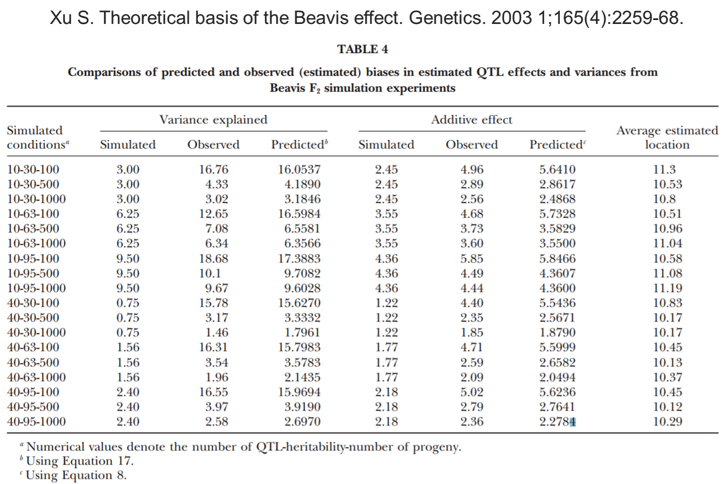
Beavis effect: 1000 is just OK

Multiple testing:

GWAS tests \(m\) hypothesis:

  • No correction: \(\alpha = 0.05\)
  • Bonferroni: \(\alpha = 0.05/m\)
  • FDR (25%): \(\alpha = 0.05/(m\times0.75)\)

Linkage mapping

  • Generally on experimental pops (F2, DH, RIL, BC)
  • Based on single-marker analysis or interval mapping
  • Recombination rates would increase power

LD mapping (or association mapping)

  • Use of historical LD between marker and QTL
  • AM allowed studies on random panels
  • Dense SNP panels would increase resolution

Structure

  1. Confounding associations with sub-populations
  2. Major limitation of association mapping
  3. Structure: PCs, clusters, subpopulation (eg. race)

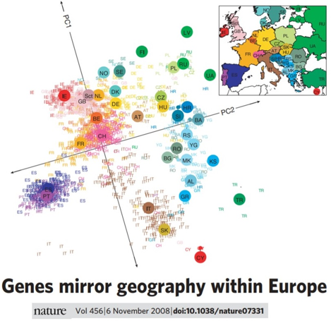
Structure

Imputation

Less missing values = more obs. = more detection power

  • Markov models: Based on flanking markers
  • Random forest: Multiple decision trees capture LD
  • kNN & Projections: Fill with similar haplotypes

GLM (generalized linear models)

  • Full model (\(L_1\)): \[y = Xb + m_ja + e\]
  • Null model (\(L_0\)): \[y = Xb + e\]
  1. Advantage: Fast, not restricted to Gaussian traits
  2. Popular methodology on human genetic studies
  3. \(Xb\) includes (1) environment, (2) structure and (3) covariates

MLM (mixed linear models)

  • Full model (\(L_1\)): \[y = Xb + Zu + m_ja + e\]
  • Null model (\(L_0\)): \[y = Xb + Zu + e\]
  1. The famous "Q+K model"
  2. Advantage: Better control of false positives, no need for PCs
  3. Polygenic effect (\(u\)) assumes \(u\sim N(0,K\sigma^2_u)\)
  4. Faster if we don't reestimate \(\lambda = \sigma^2_e/\sigma^2_u\) for each SNP

cMLM (compressed MLM)

  1. Uses the same base model as MLM
  2. Advantage: Faster than MLM
  3. Based on clustered individuals:
  • \(Z\) is indicates the subgroup
  • \(K\) is the relationship among subgroup
  • Often needs PCs to complement \(K\)

WGR (whole-genome regression)

  1. Tests all markers at once
  2. Advantage: No double-fitting, no PCs, no Bonferroni
  • Model (BayesB, BayesC, SSVS): \[y = Xb + Ma + e\]
  • Marker effects are from a mixture of distributions

\(a_j \sim Binomial\) with \(p(\pi) = 0\) and \(p(1-\pi) = a_j\)

WGR (whole-genome regression)

Rare variants

  1. Screen a set (\(s\)) of low MAF markers on NGS data
  2. Advantage: Detect signals from low power SNPs
  3. Applied to uncommon diseases (not seen in plant breeding)
  4. Two possible model
  • Full model 1 (\(L_1\)): \(y = Xb + M_sa + e\)
  • Full model 2 (\(L_2\)): \(y = Xb + PC_1(M_s) + e\)
  • Null model (\(L_0\)): \(y = Xb + e\)

Test either \(LR(L_1,L_0)\) or \(LR(L_2,L_0)\)

Validation studies

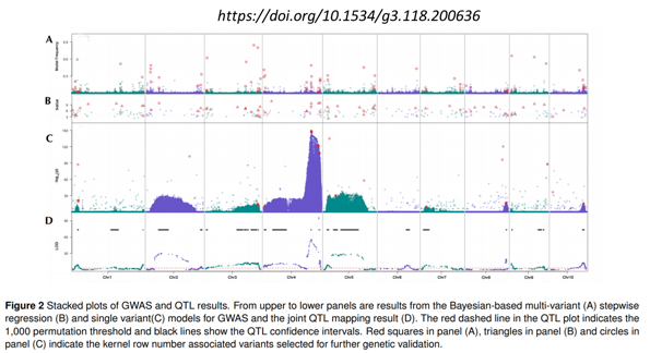
  • QTLs detected with 3 methods, across 3 mapping pops
  • Validations made on 3 unrelated populations

Break

Module 5 - Association analysis

Prelude: Data & Structure

Getting some data

Example dataset from the SoyNAM package. We are querying two of the forty biparental families with a shared parental IA3023, grown in 18 environment.

Data = SoyNAM::BLUP(trait = 'yield', family = 2:3)
## solving BLUE of checks
## solving BLUP of phenotypes
## No redundant SNPs found 
## There are 312 markers with MAF below the threshold 
## Removing markers with more than 50% missing values
## Imputing with expectation (based on transition prob) 
## removing repeated genotypes
## solving identity matrix
## indiviual 1 had 37 duplicate(s)
## indiviual 169 had 1 duplicate(s)
## indiviual 182 had 1 duplicate(s)

Genomic relationship matrix

y = Data$Phen
M = Data$Gen
#
Z = apply(M,2,function(snp) snp-mean(snp))
ZZ = tcrossprod(Z)
Sum2pq = sum(apply(M,2,function(snp){p=mean(snp)/2; return(2*p*(1-p))}))
G = ZZ/Sum2pq

Kernel commonly deployed, referred in VanRaden (2008)

\[G=\frac{(M-P)(M-p)'}{2\sum^{J}_{j=1}{p_j(1-p_j)}}\]

Genomic relationship matrix

image(G[,241:1], main='GRM heatmap',xaxt='n',yaxt='n')

Structure parameters (1) PCs

Spectral = eigen(G,symmetric = TRUE)
PCs = Spectral$vectors[,1:5]
plot(PCs,xlab='PC 1',ylab='PC 2',main='Population on eigen spaces',col=Data$Fam,pch=20)

Structure parameters (2) Clusters

GeneticDistance = Gdist(M,method=6)
## Modified Rogers' distance
Tree = hclust(GeneticDistance,method = 'ward.D2')
Clst = factor(cutree(Tree,k=2))
plot(Tree,labels = FALSE)

Single marker analysis

GLM (1) - No structure

Marker = M[,117]
#
fit = lm( y ~ Marker )
anova( fit )
## Analysis of Variance Table
## 
## Response: y
##            Df  Sum Sq Mean Sq F value    Pr(>F)    
## Marker      1  476321  476321  20.172 1.102e-05 ***
## Residuals 239 5643504   23613                      
## ---
## Signif. codes:  0 '***' 0.001 '**' 0.01 '*' 0.05 '.' 0.1 ' ' 1
-log(anova(fit)$`Pr(>F)`[1],base = 10)
## [1] 4.957736

GLM (2) - Principal Components

reduced_model = lm( y ~ PCs )
full_model = lm( y ~ PCs + Marker )
anova( reduced_model, full_model )
## Analysis of Variance Table
## 
## Model 1: y ~ PCs
## Model 2: y ~ PCs + Marker
##   Res.Df     RSS Df Sum of Sq      F    Pr(>F)    
## 1    235 4060362                                  
## 2    234 3562067  1    498295 32.734 3.215e-08 ***
## ---
## Signif. codes:  0 '***' 0.001 '**' 0.01 '*' 0.05 '.' 0.1 ' ' 1
-log((anova( reduced_model, full_model ))$`Pr(>F)`[2],base = 10)
## [1] 7.492813

GLM (3) - Population Clusters

reduced_model = lm( y ~ Clst )
full_model = lm( y ~ Clst + Marker )
anova( reduced_model, full_model )
## Analysis of Variance Table
## 
## Model 1: y ~ Clst
## Model 2: y ~ Clst + Marker
##   Res.Df     RSS Df Sum of Sq      F  Pr(>F)    
## 1    239 4275698                                
## 2    238 3652041  1    623657 40.643 9.4e-10 ***
## ---
## Signif. codes:  0 '***' 0.001 '**' 0.01 '*' 0.05 '.' 0.1 ' ' 1
-log( anova(reduced_model,full_model)$`Pr(>F)`[2],base = 10)
## [1] 9.026884

MLM - K+Q model

Q = model.matrix(~Clst)
reduced_model = reml( y=y, X=Q, K=G)
full_model = reml( y=y, X=cbind(Q, Marker), K=G)
LRT = -2*(full_model$loglik - reduced_model$loglik)
-log(pchisq(LRT,1,lower.tail=FALSE),base=10)
## [1] 10.80903

Whole genome screening

DIY (example with GLM)

reduced_model = lm( y ~ Clst )
glm_pval = apply(M,2,function(Marker){
  pval = anova(reduced_model, lm(y~Clst+Marker) )$`Pr(>F)`[2]
  return(-log(pval,base = 10))})
plot(glm_pval,pch=20,xlab='SNP',main='My first GLM GWAS')

Using CRAN implementations

NAM random model: \(y=\mu+Marker \times Pop+Zu+e\)

fit_gwa = gwas3(y=y, gen=M, fam=c(Clst), chr=Data$Chrom)
## Calculating G matrix 
## Solving polygenic model 
## Starting Eigendecomposition 
## Starting Marker Analysis 
## 
  |                                                                       
  |                                                                 |   0%
  |                                                                       
  |                                                                 |   1%
  |                                                                       
  |=                                                                |   1%
  |                                                                       
  |=                                                                |   2%
  |                                                                       
  |==                                                               |   2%
  |                                                                       
  |==                                                               |   3%
  |                                                                       
  |==                                                               |   4%
  |                                                                       
  |===                                                              |   4%
  |                                                                       
  |===                                                              |   5%
  |                                                                       
  |====                                                             |   5%
  |                                                                       
  |====                                                             |   6%
  |                                                                       
  |====                                                             |   7%
  |                                                                       
  |=====                                                            |   7%
  |                                                                       
  |=====                                                            |   8%
  |                                                                       
  |======                                                           |   8%
  |                                                                       
  |======                                                           |   9%
  |                                                                       
  |======                                                           |  10%
  |                                                                       
  |=======                                                          |  10%
  |                                                                       
  |=======                                                          |  11%
  |                                                                       
  |=======                                                          |  12%
  |                                                                       
  |========                                                         |  12%
  |                                                                       
  |========                                                         |  13%
  |                                                                       
  |=========                                                        |  13%
  |                                                                       
  |=========                                                        |  14%
  |                                                                       
  |=========                                                        |  15%
  |                                                                       
  |==========                                                       |  15%
  |                                                                       
  |==========                                                       |  16%
  |                                                                       
  |===========                                                      |  16%
  |                                                                       
  |===========                                                      |  17%
  |                                                                       
  |===========                                                      |  18%
  |                                                                       
  |============                                                     |  18%
  |                                                                       
  |============                                                     |  19%
  |                                                                       
  |=============                                                    |  19%
  |                                                                       
  |=============                                                    |  20%
  |                                                                       
  |=============                                                    |  21%
  |                                                                       
  |==============                                                   |  21%
  |                                                                       
  |==============                                                   |  22%
  |                                                                       
  |===============                                                  |  22%
  |                                                                       
  |===============                                                  |  23%
  |                                                                       
  |===============                                                  |  24%
  |                                                                       
  |================                                                 |  24%
  |                                                                       
  |================                                                 |  25%
  |                                                                       
  |=================                                                |  25%
  |                                                                       
  |=================                                                |  26%
  |                                                                       
  |=================                                                |  27%
  |                                                                       
  |==================                                               |  27%
  |                                                                       
  |==================                                               |  28%
  |                                                                       
  |===================                                              |  28%
  |                                                                       
  |===================                                              |  29%
  |                                                                       
  |===================                                              |  30%
  |                                                                       
  |====================                                             |  30%
  |                                                                       
  |====================                                             |  31%
  |                                                                       
  |====================                                             |  32%
  |                                                                       
  |=====================                                            |  32%
  |                                                                       
  |=====================                                            |  33%
  |                                                                       
  |======================                                           |  33%
  |                                                                       
  |======================                                           |  34%
  |                                                                       
  |======================                                           |  35%
  |                                                                       
  |=======================                                          |  35%
  |                                                                       
  |=======================                                          |  36%
  |                                                                       
  |========================                                         |  36%
  |                                                                       
  |========================                                         |  37%
  |                                                                       
  |========================                                         |  38%
  |                                                                       
  |=========================                                        |  38%
  |                                                                       
  |=========================                                        |  39%
  |                                                                       
  |==========================                                       |  39%
  |                                                                       
  |==========================                                       |  40%
  |                                                                       
  |==========================                                       |  41%
  |                                                                       
  |===========================                                      |  41%
  |                                                                       
  |===========================                                      |  42%
  |                                                                       
  |============================                                     |  42%
  |                                                                       
  |============================                                     |  43%
  |                                                                       
  |============================                                     |  44%
  |                                                                       
  |=============================                                    |  44%
  |                                                                       
  |=============================                                    |  45%
  |                                                                       
  |==============================                                   |  45%
  |                                                                       
  |==============================                                   |  46%
  |                                                                       
  |==============================                                   |  47%
  |                                                                       
  |===============================                                  |  47%
  |                                                                       
  |===============================                                  |  48%
  |                                                                       
  |================================                                 |  48%
  |                                                                       
  |================================                                 |  49%
  |                                                                       
  |================================                                 |  50%
  |                                                                       
  |=================================                                |  50%
  |                                                                       
  |=================================                                |  51%
  |                                                                       
  |=================================                                |  52%
  |                                                                       
  |==================================                               |  52%
  |                                                                       
  |==================================                               |  53%
  |                                                                       
  |===================================                              |  53%
  |                                                                       
  |===================================                              |  54%
  |                                                                       
  |===================================                              |  55%
  |                                                                       
  |====================================                             |  55%
  |                                                                       
  |====================================                             |  56%
  |                                                                       
  |=====================================                            |  56%
  |                                                                       
  |=====================================                            |  57%
  |                                                                       
  |=====================================                            |  58%
  |                                                                       
  |======================================                           |  58%
  |                                                                       
  |======================================                           |  59%
  |                                                                       
  |=======================================                          |  59%
  |                                                                       
  |=======================================                          |  60%
  |                                                                       
  |=======================================                          |  61%
  |                                                                       
  |========================================                         |  61%
  |                                                                       
  |========================================                         |  62%
  |                                                                       
  |=========================================                        |  62%
  |                                                                       
  |=========================================                        |  63%
  |                                                                       
  |=========================================                        |  64%
  |                                                                       
  |==========================================                       |  64%
  |                                                                       
  |==========================================                       |  65%
  |                                                                       
  |===========================================                      |  65%
  |                                                                       
  |===========================================                      |  66%
  |                                                                       
  |===========================================                      |  67%
  |                                                                       
  |============================================                     |  67%
  |                                                                       
  |============================================                     |  68%
  |                                                                       
  |=============================================                    |  68%
  |                                                                       
  |=============================================                    |  69%
  |                                                                       
  |=============================================                    |  70%
  |                                                                       
  |==============================================                   |  70%
  |                                                                       
  |==============================================                   |  71%
  |                                                                       
  |==============================================                   |  72%
  |                                                                       
  |===============================================                  |  72%
  |                                                                       
  |===============================================                  |  73%
  |                                                                       
  |================================================                 |  73%
  |                                                                       
  |================================================                 |  74%
  |                                                                       
  |================================================                 |  75%
  |                                                                       
  |=================================================                |  75%
  |                                                                       
  |=================================================                |  76%
  |                                                                       
  |==================================================               |  76%
  |                                                                       
  |==================================================               |  77%
  |                                                                       
  |==================================================               |  78%
  |                                                                       
  |===================================================              |  78%
  |                                                                       
  |===================================================              |  79%
  |                                                                       
  |====================================================             |  79%
  |                                                                       
  |====================================================             |  80%
  |                                                                       
  |====================================================             |  81%
  |                                                                       
  |=====================================================            |  81%
  |                                                                       
  |=====================================================            |  82%
  |                                                                       
  |======================================================           |  82%
  |                                                                       
  |======================================================           |  83%
  |                                                                       
  |======================================================           |  84%
  |                                                                       
  |=======================================================          |  84%
  |                                                                       
  |=======================================================          |  85%
  |                                                                       
  |========================================================         |  85%
  |                                                                       
  |========================================================         |  86%
  |                                                                       
  |========================================================         |  87%
  |                                                                       
  |=========================================================        |  87%
  |                                                                       
  |=========================================================        |  88%
  |                                                                       
  |==========================================================       |  88%
  |                                                                       
  |==========================================================       |  89%
  |                                                                       
  |==========================================================       |  90%
  |                                                                       
  |===========================================================      |  90%
  |                                                                       
  |===========================================================      |  91%
  |                                                                       
  |===========================================================      |  92%
  |                                                                       
  |============================================================     |  92%
  |                                                                       
  |============================================================     |  93%
  |                                                                       
  |=============================================================    |  93%
  |                                                                       
  |=============================================================    |  94%
  |                                                                       
  |=============================================================    |  95%
  |                                                                       
  |==============================================================   |  95%
  |                                                                       
  |==============================================================   |  96%
  |                                                                       
  |===============================================================  |  96%
  |                                                                       
  |===============================================================  |  97%
  |                                                                       
  |===============================================================  |  98%
  |                                                                       
  |================================================================ |  98%
  |                                                                       
  |================================================================ |  99%
  |                                                                       
  |=================================================================|  99%
  |                                                                       
  |=================================================================| 100%
## Calculations were performed successfully

Manhattan plot

plot(fit_gwa, pch=20, main = "My first MLM GWAS")

Yet another R implementations

require(rrBLUP,quietly = TRUE); COL = fit_gwa$MAP[,1]%%2+1 # Color chromosomes
geno=data.frame(colnames(M),fit_gwa$MAP[,1:2],t(M-1),row.names=NULL)
pheno=data.frame(line=colnames(geno)[-c(1:3)],Pheno=y,Clst,row.names=NULL)
fit_another_gwa=GWAS(pheno,geno,fixed='Clst',plot=FALSE)
## [1] "GWAS for trait: Pheno"
## [1] "Variance components estimated. Testing markers."

Comparing results

mlm_pval=fit_another_gwa$Pheno; mlm_pval[mlm_pval==0]=NA
plot(glm_pval,mlm_pval,xlab='GLM',ylab='MLM',main='Compare')

Power analysis - QQ plot

nam_pval = fit_gwa$PolyTest$pval
par(mfrow=c(1,3))
qqman::qq(glm_pval,main='GLM')
qqman::qq(mlm_pval,main='MLM')
qqman::qq(nam_pval,main='RLM')

Multiple testing

Multiple testing

Wikipedia: In statistics, the multiple comparisons, multiplicity or multiple testing problem occurs when one considers a set of statistical inferences simultaneously or infers a subset of parameters selected based on the observed values.In certain fields it is known as the look-elsewhere effect: The more inferences are made, the more likely erroneous inferences are to occur. Several statistical techniques have been developed to prevent this from happening, allowing significance levels for single and multiple comparisons to be directly compared. These techniques generally require a stricter significance threshold for individual comparisons, so as to compensate for the number of inferences being made.

Baseline - No correction

Base significance threshold: \(\alpha=0.05\)

plot(fit_gwa, alpha=0.05, main = "No correction")

Multiple testing correction

Bonferroni: \(\alpha=0.05/m\)

plot(fit_gwa, alpha=0.05/ncol(M), main = "Bonferroni correction")

False-Discovery Rate

Benjamini-Hochberg FDR: \(\alpha=\frac{0.05}{m\times (1-FDR)}\)

plot(fit_gwa, alpha=0.05/(ncol(M)*.75), main = "FDR 25%")

False-Discovery Rate

Unique segments based on Eigenvalues: \(m^* = D > 1\)

m_star = sum(Spectral$values>1)
plot(fit_gwa, alpha=0.05/m_star, main="Bonferroni on unique segments")

Multi-loci analysis

Whole genome regression

fit_wgr = bWGR::BayesDpi(y=y,X=M,it=3000); par(mfrow=c(1,2));
plot(fit_wgr$PVAL,col=COL,pch=20,ylab='-log(p)',main='GWA')
plot(fit_wgr$b,col=COL,pch=20,ylab='Marker effect',main='GWP')

plot(fit_wgr$hat,y,pch=20)

WGR - No need for multiple testing

thr_none = -log(pchisq(qchisq(1-0.05/ncol(M),1),1,lower.tail=FALSE),base=10)
thr_bonf = -log(pchisq(qchisq(1-0.05,1),1,lower.tail=FALSE),base=10)
par(mfrow=c(1,2)); plot(fit_gwa,alpha=NULL,main="MLM",pch=20); abline(h=thr_none,col=3)
plot(fit_wgr$PVAL,col=COL,ylab='-log(p)',main="WGR",pch=20); abline(h=thr_bonf,col=3)

Approaches are complementary

Random forest

fit_rf = ranger::ranger(y~.,data= data.frame(y=y,M),importance='impurity')
plot(fit_rf$variable.importance,ylab='Importance',main='Random Forest',col=COL+7,pch=20)

Thanks!

Break