- Test statistics
- Allele coding
- Power & resolution
- Linkage mapping
- LD mapping
- Structure
- Imputation
- GLM
- MLM
- WGR
- Rare-variants
- Validation studies
October 26, 2018
Outline
Test statistics
- Testing associations are as simple as t-test and ANOVA
Test statistics
- A more generalized framework: Likelihood test
\[LRT = L_0 / L_1 = -2(logL_1 - logL_0)\]
For the model:
\[y=Xb+Zu+e\\ y\sim N(Xb,V)\]
REML function is given by:
\[L(\sigma^2_u,\sigma^2_e)=-0.5( ln|V|+ln|X'V^{-1}X|+y'Py)\]
Where \(V=ZKZ'\sigma^2_u+I\sigma^2_e\) and \(y'Py=y'e\)
Allele coding
Types of allele coding
- Add. (1 df): {-1,0,1} or {0,1,2} - Very popular (Lines, GCA)
- Dom. (1 df): {0,1,0} - Popular (Trees, clonals and Hybrids)
- Jointly A+D (2 df): Popular on QTL mapping in F2s
- Complete dominance (1 df): {0,0,1} or {0,1,1} - Very unusual
- Interactions (X df): Marker x Factor (epistasis and GxE)
Power and resolution
Power
- Key: Number of individuals & allele frequency
- More DF = lower power
- Multiple testing: Bonferroni and FDR
- Tradeoff: Power vs false positives
Resolution
- Genotyping density
- LD blocks
- Recombination
Power: Variance of X
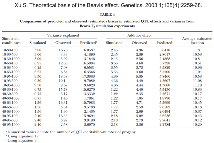
Beavis effect: 1000 is just OK

Multiple testing:
GWAS tests \(m\) hypothesis:
- No correction: \(\alpha = 0.05/m\)
- Bonferroni: \(\alpha = 0.05/m\)
- FDR (25%): \(\alpha = 0.05/(m\times0.75)\)
Linkage mapping
- Generally on experimental pops (F2, DH, RIL, BC)
- Based on single-marker analysis or interval mapping
- Recombination rates would increase power

LD mapping (or association mapping)
- Use of historical LD between marker and QTL
- AM allowed studies on random panels
- Dense SNP panels would increase resolution

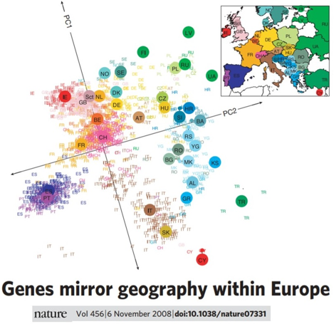
Structure
- Confounding associations with sub-populations
- Major limitation of association mapping
- Structure: PCs, clusters, subpopulation (eg. race)
Structure

Imputation
Less missing values = more obs. = more detection power
- Markov models: Based on flanking markers
- Random forest: Multiple decision trees capture LD
- kNN & Projections: Fill with similar haplotypes

GLM (generalized linear models)
- Full model (\(L_1\)): \[y = Xb + m_ja + e\]
- Null model (\(L_0\)): \[y = Xb + e\]
- Advantage: Fast, not restricted to Gaussian traits
- Popular methodology on human genetic studies
- \(Xb\) includes (1) environment, (2) structure and (3) covariates
MLM (mixed linear models)
- Full model (\(L_1\)): \[y = Xb + Zu + m_ja + e\]
- Null model (\(L_0\)): \[y = Xb + Zu + e\]
- The famous "Q+K model"
- Advantage: Better control of false positives, no need for PCs
- Polygenic effect (\(u\)) assumes \(u\sim N(0,K\sigma^2_u)\)
- Faster if we don't reestimate \(\lambda = \sigma^2_e/\sigma^2_u\) for each SNP
cMLM (compressed MLM)
- Uses the same base model as MLM
- Advantage: Faster than MLM
- Based on clustered individuals:
- \(Z\) is indicates the subgroup
- \(K\) is the relationship among subgroup
- Often needs PCs to complement \(K\)
WGR (whole-genome regression)
- Tests all markers at once
- Advantage: No double-fitting, no PCs, no Bonferroni
- Model (BayesB, BayesC, SSVS): \[y = Xb + Ma + e\]
- Marker effects are from a mixture of distributions
\(a_j \sim Binomial\) with \(p(\pi) = 0\) and \(p(1-\pi) = a_j\)
WGR (whole-genome regression)
Rare variants
- Screen a set (\(s\)) of low MAF markers on NGS data
- Advantage: Detect signals from low power SNPs
- Applied to uncommon diseases (not seen in plant breeding)
- Two possible model
- Full model 1 (\(L_1\)): \(y = Xb + M_sa + e\)
- Full model 2 (\(L_2\)): \(y = Xb + PC_1(M_s) + e\)
- Null model (\(L_0\)): \(y = Xb + e\)
Test either \(LR(L_1,L_0)\) or \(LR(L_2,L_0)\)
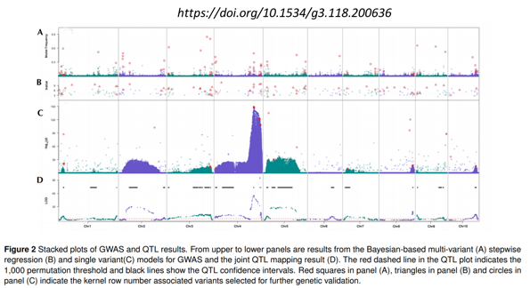
Validation studies
- QTLs detected with 3 methods, across 3 mapping pops
- Validations made on 3 unrelated populations
