final_project
Tiana Bell
8/10/2018
The Data
The American Time Use Survey (ATUS) is a time-use survey of Americans, which is sponsored by the Bureau of Labor Statistics (BLS) and conducted by the U.S. Census Bureau. Respondents of the survey are asked to keep a diary for one day carefully recording the amount of time they spend on various activities including working, leisure, childcare, and household activities. The survey has been conducted every year since 2003.
Included in the data are main demographic variables such as respondents’ age, sex, race, marital status, and education. The data also includes detailed income and employment information for each respondent. While there are some slight changes to the survey each year, the main questions asked stay the same. You can find the data dictionaries for each year on https://www.bls.gov/tus/dictionaries.htm
Accessing the Data
There are multiple ways to access the ATUS data; however, for this project, you’ll get the raw data directly from the source. The data for each year can be found at https://www.bls.gov/tus/#data. Once there, there is an option of downloading a multi-year file, which includes data for all of the years the survey has been conducted, but for the purposes of this project, let’s just look at the data for 2016. Under Data Files, click on American Time Use Survey--2016 Microdata files.
You will be brought to a new screen. Scroll down to the section 2016 Basic ATUS Data Files. Under this section, you’ll want to click to download the following two files: ATUS 2016 Activity summary file (zip) and ATUS-CPS 2016 file (zip).
ATUS 2016 Activity summary file (zip)contains information about the total time each ATUS respondent spent doing each activity listed in the survey. The activity data includes information such as activity codes, activity start and stop times, and locations.ATUS-CPS 2016 file (zip)contains informaton about each household member of all individuals selected to participate in the ATUS.
Once they’ve been downloaded, you’ll need to unzip the files. Once unzipped, you will see the dataset in a number of different file formats including .sas, .sps, and .dat files. We’ll be working with the .dat files.
Loading the Data into R
Use the first approach explained above to download and access the ATUS data for 2016. Download the CPS and Activity Summary files in a folder and unzip them and within each folder upload the files ending in .dat to data/raw_data folder on RStudio.cloud. To load the data in, run the code in the atus-data code chunk to create an object called atus.all.
Importing data
#load data from data files onto the workspace
atus.cps <- read.delim('/cloud/project/final_project/data/raw_data/atuscps_2016.dat', sep=",")
atus.sum <- read.delim('/cloud/project/final_project/data/raw_data/atussum_2016.dat', sep=",")
# joining all three files together by respondents' ID
atus.all <- atus.sum %>%
  left_join(atus.cps %>% filter(TULINENO==1), by = c("TUCASEID"))
Exploratory Analysis of Child Care Data
### general exploratory code
str(atus.all)
summary(atus.all)
colnames(atus.all)
rownames(atus.all)
## find average amount of time person spends doing "t120101"
mean(atus.all$t120101)## [1] 38.06481## write out al columns up to t030112 for sum of CHILDCARE column.
atus.all <- atus.all %>%
mutate(CHILDCARE = t030101 + t030102 + t030103 + t030104 + t030105 + t030106 + t030108 + t030109 + t030110 + t030111 + t030112 %>%
glimpse(CHILDCARE))Creating new column.
childcare_density_plot <- ggplot(atus.all, aes(CHILDCARE, na.rm = FALSE)) +
    geom_density()
This graph shows us the respondents that correlate with the amount of time spent with their children.
#this chart will show the average for the amount of time men and women spend with children.
#pull from the desired data frame
atus.all %>%
  #group by variable you are trying to isolate, in this case gender
    group_by(TESEX) %>%
  #create a variable to get expected outcome
   summarise(avg_parent_childcare = mean(CHILDCARE))
## # A tibble: 2 x 2
## TESEX avg_parent_childcare
## <int> <dbl>
## 1 1 19.0
## 2 2 33.1In this analysis we can tell that males(variable = 1) spend on average 19 mins with children compared to females (variable = 2) that spend on average 33 minutes with children. These numbers are a reflection of individual respondents without other factors(i.e. marital status, age, etc.).
#exclude all missing factors
## replace -1 in the variable TRDPFTPT with NA.
  atus.all$TRDPFTPT[atus.all$TRDPFTPT == -1] <- NA %>%
  sum(is.na(atus.all$TRDPFTPT))##take this away, filter once done.
grep("TRHHCHILD",names(atus.all))
## integer(0)#find the amount of missing values in the column
sum(is.na(atus.all$TRDPFTPT))## [1] 4119class(atus.all$TRYHHCHILD)## [1] "integer"The next thing to do is to do some substitutions in how we want missing values to be read in certain columns and data frames. This step helps reduce confusion as well as unneeded data that may mess up future graphs or equations. In this particular code chunk we are telling the computer that we want every NA *(which means missing value)* to be a -1 in the TRDPFTPT column. This will also change the class of our column.
## do younger people spend more time with children than older people.
adults_atLeast_one_kid <- atus.all %>%
  select(CHILDCARE, TEAGE, TRYHHCHILD, HEFAMINC, TRCHILDNUM, PEMARITL, TRDPFTPT, TESEX) %>%
       filter(TRCHILDNUM >  0)

 ggplot(adults_atLeast_one_kid, aes(x = TEAGE, y = CHILDCARE)) +
      geom_point(aes(color = factor(TEAGE)), size = 1) +
      theme(legend.position = "none") +
      labs( x = "RESPONDENT'S AGE \n years", y = "CHILDCARE \n minutes per week", title = "Do younger people spend more time with \n their children than older people?")
In this graph we are answering the question of whether younger respondents spend more time with children than with older respondents.* Since our data set are respondents between the ages 15 to around 85, our dividing(median) age is 50. By looking at the chart you can see that individuals below 50 spend more time with their children than those older than them. It is also colored by respondents’ marital status.
** Note that this data only includes respondents with at least one child within the household that they take care of. And this variable will stay constant for the next three graphs!**
## do richer people spend more time with children than poor
      ggplot(adults_atLeast_one_kid, aes(x = HEFAMINC, y = CHILDCARE, col = TESEX )) +
      geom_point(aes(color = factor(TEAGE)), size = 1) +
      theme(legend.position = "none") +
      labs( x = "FAMILY INCOME \n tens of thousands", y = "CHILDCARE \n minutes per week", title = "Do affluent respondents spend more time with \n their children than non-affluent respondents?")
In this graph we can see that a respondent’s income* does not necessarily affect the amount of time spent with their respective child, other than the obvious outliers within each tax bracket. Although you can see a slight rise, or peak, after the 12th tax bracket! The colors are by age.
* Income key: + 1 Less than $5,000 + 2 $5,000 to $7,499 + 3 $7,500 to $9,999 + 4 $10,000 to $12,499 + 5 $12,500 to $14,999 + 6 $15,000 to $19,999 + 7 $20,000 to $24,999 + 8 $25,000 to $29,999 + 9 $30,000 to $34,999 + 10 $35,000 to $39,999 + 11 $40,000 to $49,999 + 12 $50,000 to $59,999 + 13 $60,000 to $74,999 + 14 $75,000 to $99,999 + 15 $100,000 to $149,999 + 16 $150,000 and over
*Note that income is based on household, not individual respondent.*
## do married people spend more time with children than single parents
      ggplot(adults_atLeast_one_kid, aes(x = factor(PEMARITL), y = CHILDCARE, fill = factor(PEMARITL))) +
         geom_bar(stat = "identity") +
         labs( x = "Marital Status", y = "CHILDCARE \n minutes per week", title = "Do married people spend more time with \n their children than single people?")
With the Marital Status Key* in mind *(see below)*, we can see that married respondents with the spouse present on average spend more time with their children than any of the other categories of respondents.
*Martial Status Key: + 1 Married - spouse present + 2 Married - spouse absent + 3 Widowed + 4 Divorced + 5 Separated + 6 Never married
 filter(adults_atLeast_one_kid, !is.na(TRDPFTPT)) %>%
## do full-time workers spend more time than part-time workers?
      ggplot(aes(x = factor(TRDPFTPT), y = CHILDCARE, color = factor(TRDPFTPT))) +
        geom_point() +
         labs( x = "Employment Status", y = "CHILDCARE \n minutes per week", title = "Do full-time workers spend more time with \n their children than part-time workers?")
We can see that full-time workers *(represented by 1)* spend more time with children than part-time workers *(represented by 2)*.
Regression Analysis
## add your regression analysis code here
adults_atLeast_one_kid <- lm(CHILDCARE ~ TEAGE + HEFAMINC + PEMARITL + TRDPFTPT + TESEX, data = adults_atLeast_one_kid)
summary(adults_atLeast_one_kid)
##
## Call:
## lm(formula = CHILDCARE ~ TEAGE + HEFAMINC + PEMARITL + TRDPFTPT +
## TESEX, data = adults_atLeast_one_kid)
##
## Residuals:
## Min 1Q Median 3Q Max
## -109.01 -54.65 -31.53 24.05 721.39
##
## Coefficients:
## Estimate Std. Error t value Pr(>|t|)
## (Intercept) 109.4030 12.3262 8.876 < 2e-16 ***
## TEAGE -1.6735 0.1721 -9.726 < 2e-16 ***
## HEFAMINC 0.6144 0.4771 1.288 0.198
## PEMARITL -7.9500 0.9465 -8.400 < 2e-16 ***
## TRDPFTPT -4.1119 4.1369 -0.994 0.320
## TESEX 21.3065 3.3862 6.292 3.57e-10 ***
## ---
## Signif. codes: 0 '***' 0.001 '**' 0.01 '*' 0.05 '.' 0.1 ' ' 1
##
## Residual standard error: 89.76 on 3116 degrees of freedom
## (1191 observations deleted due to missingness)
## Multiple R-squared: 0.04988, Adjusted R-squared: 0.04835
## F-statistic: 32.71 on 5 and 3116 DF, p-value: < 2.2e-16Exploratory Analysis of Age and Activities
## select
atus.wide <- atus.all %>%
    mutate(act01 = rowSums(atus.all[,grep("t01", names(atus.all))]),
           act02 = rowSums(atus.all[,grep("t02", names(atus.all))]),
           act03 = rowSums(atus.all[,grep("t03", names(atus.all))]),
           act04 = rowSums(atus.all[,grep("t04", names(atus.all))]),
           act05 = rowSums(atus.all[,grep("t05", names(atus.all))]),
           act06 = rowSums(atus.all[,grep("t06", names(atus.all))]),
           act07 = rowSums(atus.all[,grep("t07", names(atus.all))]),
           act08 = rowSums(atus.all[,grep("t08", names(atus.all))]),
           act09 = rowSums(atus.all[,grep("t09", names(atus.all))]),
           act10 = rowSums(atus.all[,grep("t10", names(atus.all))]),
           act11 = rowSums(atus.all[,grep("t11", names(atus.all))]),
           act12 = rowSums(atus.all[,grep("t12", names(atus.all))]),
           act13 = rowSums(atus.all[,grep("t13", names(atus.all))]),
           act14 = rowSums(atus.all[,grep("t14", names(atus.all))]),
           act15 = rowSums(atus.all[,grep("t15", names(atus.all))]),
           act16 = rowSums(atus.all[,grep("t16", names(atus.all))]),
           # act17 = , there is no category 17 in the data
           act18 = rowSums(atus.all[,grep("t18", names(atus.all))])) %>%
    select(TUCASEID, TEAGE, HEFAMINC, starts_with("act"))

    head(atus.wide)
## TUCASEID TEAGE HEFAMINC act01 act02 act03 act04 act05 act06 act07
## 1 2.01601e+13 62 3 715 190 0 0 0 0 0
## 2 2.01601e+13 69 6 620 230 0 0 0 0 0
## 3 2.01601e+13 24 4 1060 105 0 0 0 0 60
## 4 2.01601e+13 31 8 655 395 60 0 0 0 0
## 5 2.01601e+13 59 13 580 250 0 0 0 0 18
## 6 2.01601e+13 16 5 620 100 0 0 0 0 0
## act08 act09 act10 act11 act12 act13 act14 act15 act16 act18
## 1 0 0 0 40 465 0 0 0 0 30
## 2 0 0 0 30 560 0 0 0 0 0
## 3 0 0 0 75 20 0 0 0 0 60
## 4 0 0 0 165 120 0 0 0 45 0
## 5 0 0 0 30 177 0 60 130 120 75
## 6 0 0 0 120 355 50 0 0 0 35df.long <- atus.wide %>%
# use code to convert the wide format to long.
gather(ACTIVITY, MINS, act01:act18)
head(df.long)## TUCASEID TEAGE HEFAMINC ACTIVITY MINS
## 1 2.01601e+13 62 3 act01 715
## 2 2.01601e+13 69 6 act01 620
## 3 2.01601e+13 24 4 act01 1060
## 4 2.01601e+13 31 8 act01 655
## 5 2.01601e+13 59 13 act01 580
## 6 2.01601e+13 16 5 act01 620# Plot for average amount of time spent by age!
# pull from the desired data set, in this case we are working with df.long
df.long %>%
# follow the instructions and grouby() Activity and age
group_by(ACTIVITY, TEAGE) %>%
# calculate the average amount of time people spend on each activity
summarise(AVGMINS = mean(MINS)) %>%
# Plot the graph!
ggplot(aes(x = TEAGE, y = AVGMINS)) +
geom_bar(stat = "identity", aes(color = factor(TEAGE)))+
facet_grid(rows = vars(ACTIVITY)) +
coord_flip()+
labs( title = "Average amount of time spent \n per person's age") +
theme(text = element_text(size=18),
axis.text.x = element_text(angle=90, hjust=1))
We were asked to plot the respondent’s age against the average amount of time for each activity provided! We are asked the question : Which categories does the average time spent vary by age?
In this plot we can see that activities 1, 5, and 12, vary by age!
Exploratory Analysis of Income and Activities
activity_by_income <-df.long %>%
  group_by(ACTIVITY, HEFAMINC) %>%
  ## add the rest of the code here
  summarise(AVGMINS_WRK = mean(MINS)) %>%
  #create new colummn to set y-axis equal from 0 to 1 for proportions
  mutate(SumMins = sum(AVGMINS_WRK)) %>%
  #divide the new column by the average to create percentafe proportions
  mutate(AvgSumMins = AVGMINS_WRK/SumMins)%>%
  #plot the graph
  ggplot(aes(x = ACTIVITY,y = AvgSumMins)) +
    geom_bar(stat = "identity", aes(fill = factor(HEFAMINC))) +
        scale_fill_hue(h = c(180, 450)) +
        coord_flip()+
         labs(title = "Amount of time spent on activities \n by income")

activity_by_income
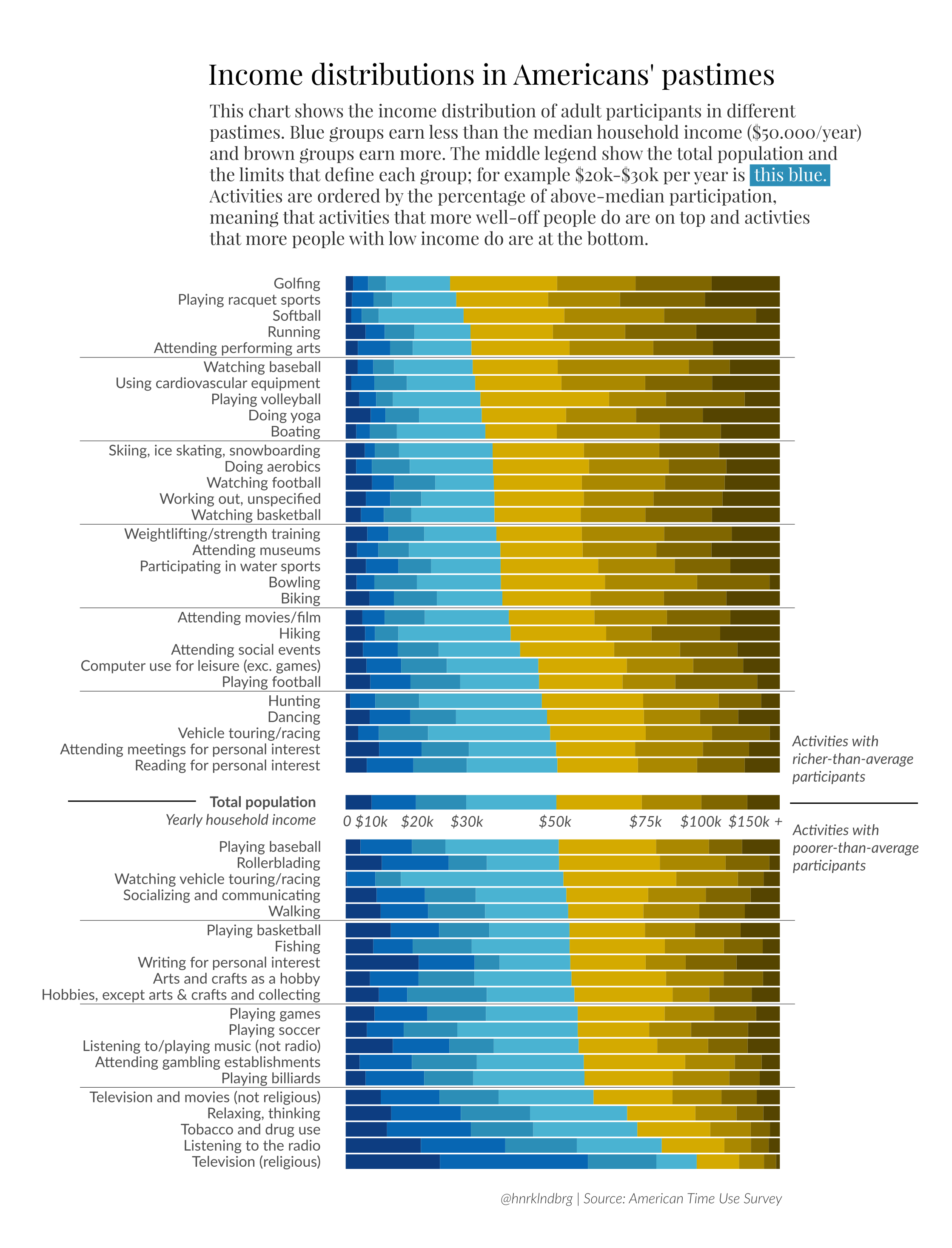
In this graph I was trying to imitate what Henrik Lindberg did in his analysis of Income distributions in America’s pastimes https://raw.githubusercontent.com/halhen/viz-pub/master/pastime-income/pastime.png. I am able to properly graph, but I am unable to get the proportions correctly!
## save the plot above
ggsave(filename = "activity_by_income.png", plot = last_plot(), path = "/cloud/project/final_project/figures/explanatory_figures" )
## Saving 7 x 5 in image