Deep Learning with R using TensorFlow via Keras

Leon Eyrich Jessen, PhD
August 21st 2018

plot of chunk unnamed-chunk-1

Postdoctoral Researcher
Immunoinformatics and Machine Learning group
Department of Bio and Health Informatics
Technical University of Denmark

Talk
Department of Food Science
University of Copenhagen

@jessenleon

Who am I?

plot of chunk unnamed-chunk-6

  • My name is Leon Eyrich Jessen
  • I have a background in wet lab biotech engineering (Think pipettes, goggles and lab coats)
  • and a PhD in Bioinformatics (I will get back to what that is)
  • I am a currently a Postdoctoral Researcher (What you do after your PhD, when you're too scared of the real world)
  • I am in the Immunoinformatics and Machine Learning Group at the Technical University of Denmark
  • I teach Introductory Data Science, Immunological Bioinformatics and I do guest lectures and workshops on deep learning at university at master level

So you do Bioinformatics - What is that?

  • Bioinformatics is Data Science with domain specific knowledge in Biology

plot of chunk unnamed-chunk-7

...and more specifically, I actually do Immunoinformatics

  • I use neural networks to model molecular interactions in the human immune system in context of infectious diseases and cancer

plot of chunk unnamed-chunk-8

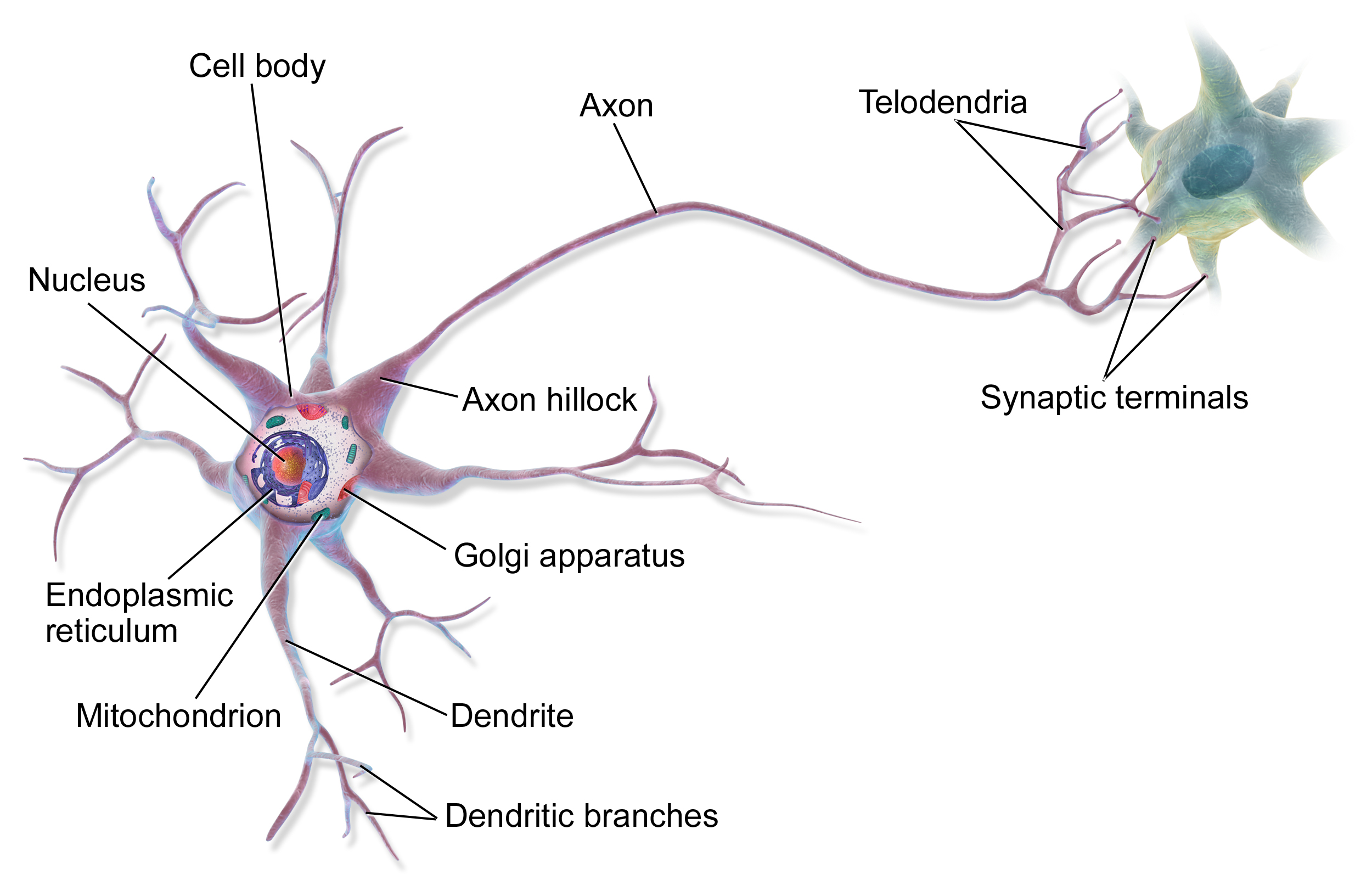
What are Artificial Neural Networks?

  • A mathematical framework for mimicking how the human brain processes data
  • The human brain consists of 100.000.000.000 cells
  • Together they form an intrigate network
  • Through hundreds of thousands of years, evolution has fine tuned our brain for one purpose: Processing massive amounts of data in real time!
  • Our brains processes vision, smell, taste, sound and physical touches in order for you to exist and interact with the world - All of which is happening inside you right now!
  • Think about it, our brain is a data center! (I think that's super cool!)

Basic Feed Forward Multilayer Perceptron - Architecture

  • Fully connected dense neural network wih one input layer, one hidden layer and one output neuron

plot of chunk unnamed-chunk-10

  • Based on input, the neuron has to 'decide' whether to send a signal via the axon or not

plot of chunk unnamed-chunk-11

Source: Bruce Blaus | Multipolar Neuron | CC BY 3.0

Why are artificial neural networs so powerful?

  • ANNs can identify context dependence!
  • I.e. the “meaning” of each variable depends not only on its observed value, but also on the context in which it was observed!
  • I bet you can read this word quite easily, but take a closer look

plot of chunk unnamed-chunk-12

Keras and TensorFlow - What you need to know

  • TensorFlow is an open source software library for numerical computations written in C++ (I.e. not confined to ANNs)
  • Originally developed by researchers and engineers working on the Google Brain team within Google's Machine Intelligence Research organization for the purposes of conducting machine learning and deep neural networks research
  • The core TensorFlow API is written in Python
  • Keras is a high-level neural networks API, written in Python running on top of TensorFlow (or CNTK or Theano)
  • Keras was developed by by François Chollet with a focus on enabling fast experimentation “Being able to go from idea to result with the least possible delay is key to doing good research”
  • The Keras R-package is written in R by François Chollet and JJ Allaire
  • The Keras interface is a really nice high level vocabulary for doing deep learning that fits really well with the way R-users work and think
  • JJ Allaire has stated that “I have my heart in getting Keras and TensorFlow to work really really well in Deep Learning in R and hook into the RStudio IDE”
  • The Keras R API calls the Keras Python API, which calls the core Python TensorFlow API which calls the TensorFlow C++ library
  • Granted, a bit complicated, but my experience so far is, that it works

Sources: keras.io, tensorflow.rstudio.com, github.com/tensorflow, keras.rstudio.com, Machine Learning with R and TensorFlow, TensorFlow and Keras in R - Josh Gordon meets with J.J. Allaire

Let us get to it - Installing Keras and TensorFlow

Installing Keras and TensorFlow

Using Hadley Wickham's devtools, it is straightforward to install both keras and TensorFlow:

install.packages('devtools')
devtools::install_github("rstudio/keras")
library("keras")
install_keras()

Hereafter all we will need to do, is run

library("keras")

That's it! Now we're ready to do deep learning in R!

A Couple of Examples

Example 1: Three-Class Classifier using the Classic Iris data set and Keras/TensorFlow

(Because it's R and we have to use either mtcars or iris)

The Iris data set

  • The famous Iris flower data set contains data to quantify the morphologic variation of Iris flowers of three related species.
  • 150 observations
  • 4 input features Sepal.Length, Sepal.Width, Petal.Length and Petal.Width
  • 3 output classes setosa versicolor and virginica
  • Balanced data with 50 observations in each class

plot of chunk unnamed-chunk-15

The Iris data set

  • We can do a simple dimension reduction using PCA to get an impression of the the degree of separation inbetween the three classes:
  • setosa is clearly separated, whereas versicolor and virginica seem more intertwined
  • Nearly all of the variance are explained by PC1 and PC2

plot of chunk unnamed-chunk-16

Neural Network Classifier Model

Here is an illustration of the model we will be building with 35 parameters, i.e. \( (n_{features} + 1) \cdot m_{hidden} + (m_{hidden} + 1) \cdot l_{output} \)

plot of chunk unnamed-chunk-17

Prepare data

We start with slightly wrangling the iris data set by renaming and scaling the features and converting character labels to numeric:

nn_dat = iris %>% as_tibble %>%
  mutate(sepal_l_feat = scale(Sepal.Length),
         sepal_w_feat = scale(Sepal.Width),
         petal_l_feat = scale(Petal.Length),
         petal_w_feat = scale(Petal.Width),          
         class_num    = as.numeric(Species) - 1, # factor, so = 0, 1, 2
         class_label  = Species) %>%
  select(contains("feat"), class_num, class_label)
nn_dat
# A tibble: 150 x 6
   sepal_l_feat sepal_w_feat petal_l_feat petal_w_feat class_num
          <dbl>        <dbl>        <dbl>        <dbl>     <dbl>
 1       -0.898       1.02          -1.34        -1.31         0
 2       -1.14       -0.132         -1.34        -1.31         0
 3       -1.38        0.327         -1.39        -1.31         0
 4       -1.50        0.0979        -1.28        -1.31         0
 5       -1.02        1.25          -1.34        -1.31         0
 6       -0.535       1.93          -1.17        -1.05         0
 7       -1.50        0.786         -1.34        -1.18         0
 8       -1.02        0.786         -1.28        -1.31         0
 9       -1.74       -0.361         -1.34        -1.31         0
10       -1.14        0.0979        -1.28        -1.44         0
# ... with 140 more rows, and 1 more variable: class_label <fct>

Here, we use scaling such that the mean of each feature is 0 and the standard deviation is 1

Scaling

Feature distributions before scaling

plot of chunk unnamed-chunk-19

Feature distributions after scaling

plot of chunk unnamed-chunk-20

Prepare data

Then, we split the iris data into a training and a test data set, setting aside 20% of the data for left out data partition, to be used for final performance evaluation:

test_f = 0.20
nn_dat = nn_dat %>%
  mutate(partition = sample(c('train','test'), nrow(.), replace = TRUE, prob = c(1 - test_f, test_f)))

Based on the partition, we can now create training and test data, where x is a matrix and y is the one-hot encoding of the category

x_train = nn_dat %>% filter(partition == 'train') %>% select(contains("feat")) %>% as.matrix
y_train = nn_dat %>% filter(partition == 'train') %>% pull(class_num)          %>% to_categorical
x_test  = nn_dat %>% filter(partition == 'test')  %>% select(contains("feat")) %>% as.matrix
y_test  = nn_dat %>% filter(partition == 'test')  %>% pull(class_num)          %>% to_categorical

Thereby yielding

x_train %>% head(3)
     sepal_l_feat sepal_w_feat petal_l_feat petal_w_feat
[1,]   -0.8976739   1.01560199    -1.335752    -1.311052
[2,]   -1.5014904   0.09788935    -1.279104    -1.311052
[3,]   -1.0184372   0.78617383    -1.279104    -1.311052
y_train %>% head(3)
     [,1] [,2] [,3]
[1,]    1    0    0
[2,]    1    0    0
[3,]    1    0    0

Set Architecture, Compile Model and Train Classifier

With the data in place, we now set the architecture of our artificical neural network:

model = keras_model_sequential()
model %>% 
  layer_dense(units = 4, activation = 'sigmoid', input_shape = 4) %>% 
  layer_dense(units = 3, activation = 'softmax')

Where \( softmax(x_i) = \frac{ e^{x_i} }{ \sum_{i=1}^{n} e^{x_i} } \), such that \( \sum(softmax(x)) = 1 \)

Then we compile our model:

model %>% compile(
  loss      = 'categorical_crossentropy',
  optimizer = optimizer_rmsprop(),
  metrics   = c('accuracy')
)

and finally, we train our classifier

history = model %>% fit(
  x = x_train, y = y_train,
  epochs           = 200,
  batch_size       = 20,
  validation_split = 0,
  view_metrics     = FALSE,
  verbose = 0
)

Visualise training

The fit() function returns a history object, which we can plot like so

plot(history)

plot of chunk unnamed-chunk-28

Evaluate Model Performance

We can use the evaluate() function, to get the loss and accuracy metrics from the model

perf = model %>% evaluate(x_test, y_test)
print(perf)
$loss
[1] 0.3366045

$acc
[1] 0.972973

Predict on New Data

We can use the predict() and predict_classes() function for predicting soft and hard classifications respectively:

model %>% predict(x_test) %>% head
          [,1]       [,2]        [,3]
[1,] 0.8970004 0.09539866 0.007600991
[2,] 0.9257328 0.06898528 0.005281978
[3,] 0.9348749 0.06047851 0.004646669
[4,] 0.9333495 0.06154421 0.005106285
[5,] 0.9334606 0.06181232 0.004727044
[6,] 0.9097174 0.08376918 0.006513394
model %>% predict_classes(x_test) %>% head
[1] 0 0 0 0 0 0

Confusion Matrix Visualisation

…and finally we can visualise the confusion matrix based on the original 20% left out test data

plot of chunk unnamed-chunk-31

Example 2: Modelling Molecular Interactions

Very Brief Background

  • The basic living unit of our body is a cell
  • Inside the cell DNA is being translated to proteins
  • Inside the cell, proteins are needed to make the cell function
  • Small fragments of proteins called peptides from inside the cell are constantly being transported to the outside and presented for immune cells to monitor the health if the cell
  • The basic building block of a protein is an amino acid
  • All proteins in the human body are build from only 20 amino acids
  • In the following, we will model if a peptide will or will not bind to the presenter-protein

plot of chunk unnamed-chunk-32

Figure by Eric A. J. Reits

Cancer Immunotherapy

  • Cancer “happens”, when cells of our body go out of control
  • Cancer Immunotherapy is a cancer treatment strategy, where the aim is to utilize the cancer patient’s own immune system to fight the cancer
  • The health system of a cancer cell is different than that of a non-sick cell
  • This difference can be detected by our immune system
  • However, the environment around the cancer cells is very hostile to the immune system
  • Therefore, we can extract immune cells and predict their cancer-target, grow them in great numbers and re-introduce them in the patient
  • Or, we can engineer immune cells to react to a specific target and then grow them in great numbers and re-introduce them in the patient
  • Either way we need to know what are the cancer-targets and which immune cells will hit that target
  • Enter Deep Learning for modelling molecular interactions!

Data

  • The peptide data set we will be working with consists of 7,920 positives and 7,920 negatives randomly split into 6 partitions:
pep_dat
# A tibble: 15,840 x 3
   peptide   binder partition
   <chr>      <int>     <int>
 1 LLTDAQRIV      0         1
 2 LMAFYLYEV      1         4
 3 VMSPITLPT      0         1
 4 SLHLTNCFV      0         5
 5 RQFTCMIAV      0         3
 6 FMNGHTHIA      1         2
 7 KINPYFSGA      0         3
 8 NIWLAIIEL      0         1
 9 KIMPYVAQF      0         2
10 AIWERACTI      0         3
# ... with 15,830 more rows
  • The peptide variable, where the first observation is LLTDAQRIV is what we will use as input to our model (Each letter represents an amino acid)
  • All peptides consist of 9 amino acids
  • Each amino acid is converted (encoded) to a vector of 21 numbers based on its bio-chemical properties

Data

After encoding, each peptide is in essense converted to an image, i.e. a numeric representation of the biochemical profile of the peptide

pep_plot_encoding(pep = 'LLTDAQRIV')

plot of chunk unnamed-chunk-36

Data

We will use partition 6 as independent test set and then do 5-fold cross validation on partitions 1 through 5

pep_dat_test_set = pep_dat %>% filter(partition == 6)
pep_dat = pep_dat %>% filter(partition != 6)
partitions  = pep_dat %>% count(partition) %>% pull(partition) # 1 2 3 4 5
data_splits = cross_fold_splits(partitions = partitions, print_splits = TRUE)
________________________________________________________________________________
Based on (1, 2, 3, 4, 5), the following 20 splits were created:
________________________________________________________________________________
Test partition = 1, Validation partition = 2, Training partitions = 3, 4, 5
Test partition = 1, Validation partition = 3, Training partitions = 2, 4, 5
Test partition = 1, Validation partition = 4, Training partitions = 2, 3, 5
Test partition = 1, Validation partition = 5, Training partitions = 2, 3, 4
Test partition = 2, Validation partition = 1, Training partitions = 3, 4, 5
Test partition = 2, Validation partition = 3, Training partitions = 1, 4, 5
Test partition = 2, Validation partition = 4, Training partitions = 1, 3, 5
Test partition = 2, Validation partition = 5, Training partitions = 1, 3, 4
Test partition = 3, Validation partition = 1, Training partitions = 2, 4, 5
Test partition = 3, Validation partition = 2, Training partitions = 1, 4, 5
Test partition = 3, Validation partition = 4, Training partitions = 1, 2, 5
Test partition = 3, Validation partition = 5, Training partitions = 1, 2, 4
Test partition = 4, Validation partition = 1, Training partitions = 2, 3, 5
Test partition = 4, Validation partition = 2, Training partitions = 1, 3, 5
Test partition = 4, Validation partition = 3, Training partitions = 1, 2, 5
Test partition = 4, Validation partition = 5, Training partitions = 1, 2, 3
Test partition = 5, Validation partition = 1, Training partitions = 2, 3, 4
Test partition = 5, Validation partition = 2, Training partitions = 1, 3, 4
Test partition = 5, Validation partition = 3, Training partitions = 1, 2, 4
Test partition = 5, Validation partition = 4, Training partitions = 1, 2, 3
________________________________________________________________________________

About Cross Validation

  • Cross validation is a procedure for avoiding overfitting, so that the final model can extrapolate on unseen data
  • In this case we
    • Split the data into 5 subsets randomly
    • Model 1 will use partition 1 as unseen test set and will train on partitions 3,4,5 until best possible performance is obtained on partition 2
    • Model 2 will use partition 1 as unseen test set and will train on partitions 2,4,5 until best possible performance is obtained on partition 3
    • Model 3 will use partition 1 as unseen test set and will train on partitions 2,3,5 until best possible performance is obtained on partition 4
    • Model 20 will use partition 5 as unseen test set and will train on partitions 1,2,3 until best possible performance is obtained on partition 4
  • (Technically, this is actually 5-fold nested cross validation)

plot of chunk unnamed-chunk-39

Defining and Compiling the Model

Set hyper parameters

model_activation    = "sigmoid"
model_learning_rate = 0.0001
model_optimizer     = optimizer_adam(lr = model_learning_rate)
model_loss          = 'mean_squared_error'
model_metrics       = 'mean_squared_error'
model_epochs        = 10
model_batch_size    = 20
model_layer_IN_n    = 189 # 9 amino acids x 21 enc values
model_layer_H1_n    = 189
model_layer_H2_n    = 90
model_layer_H3_n    = 45
model_layer_OUT_n   = 1   # Is the peptide a binder (yes/no)

Set architecture

model = keras_model_sequential() %>% 
  layer_dense(units = model_layer_H1_n,  activation = model_activation, input_shape = model_layer_IN_n) %>% 
  layer_dense(units = model_layer_H2_n,  activation = model_activation) %>%
  layer_dense(units = model_layer_H3_n,  activation = model_activation) %>%
  layer_dense(units = model_layer_OUT_n, activation = model_activation)

Compiling the model

model %>% compile(loss = model_loss, optimizer = model_optimizer, metrics = model_metrics)

Note! The 20 splits result in our final model consisting of 20 models, each of which have 57,151 parameters. Together they form an ensembl model with roughly 1,15 million parameters!

Training the model

meta_data = list()
model_dir = 'models/'
for( mdl_i in names(data_splits) ){
  # Set partitions
  test_partition       = data_splits[[mdl_i]]$test_partition
  validation_partition = data_splits[[mdl_i]]$validation_partition
  training_partitions  = data_splits[[mdl_i]]$training_partitions

  # Set model file
  mdl_file = str_c(model_dir, mdl_i, ".hdf5")

  # Set callbacks used for early stopping
  callbacks_list = list( callback_early_stopping(monitor = "mean_squared_error", patience = 10),
                         callback_model_checkpoint(filepath = mdl_file, monitor = "val_loss",
                                                   save_best_only = TRUE) )
  # Extract and encode current training data
  pep_dat_training = pep_dat %>% filter(partition %in% training_partitions)
  x_train          = pep_dat_training %>% pull(peptide) %>% pep_encode(mat = "BLOSUM50") %>%
    array_reshape(c(dim(.)[1], dim(.)[2] * dim(.)[3]))
  y_train          = pep_dat_training %>% pull(binder) %>% array

  # Extract and encode current validation data
  pep_dat_validation = pep_dat %>% filter(partition %in% validation_partition)
  x_validation       = pep_dat_validation %>% pull(peptide) %>% pep_encode(mat = "BLOSUM50") %>%
    array_reshape(c(dim(.)[1], dim(.)[2] * dim(.)[3]))
  y_validation       = pep_dat_validation %>% pull(binder) %>% array

  # Do training
  history = model %>% fit(x = x_train, y = y_train, batch_size = model_batch_size, epochs = model_epochs,
                          callbacks = callbacks_list, validation_data = list(x_validation, y_validation))
  # Save meta data
  meta_data[[mdl_i]] = list(); meta_data[[mdl_i]]$mdl_file = mdl_file ; meta_data[[mdl_i]]$history = history
}

Add Predictions to the Peptide Data Set

For each of the 20 models, we can now add predictions on the corresponding test set

for( mdl_id in names(meta_data) ){

  # Load current model  
  mdl = load_model_hdf5(filepath = meta_data[[mdl_id]]$mdl_file)
  meta_data[[mdl_id]]$model = mdl

  # Do prediction. Note how prediction are ONLY made for data points from the
  # test partition of the current model!
  pred_id = str_c('pred_', mdl_id)
  pep_dat = pep_dat %>% 
    mutate(!!pred_id := ifelse( partition == data_splits[[mdl_id]]$test_partition,
      pep_predict(peptide = peptide, model = mdl), NA))

}
# Calculate mean predictions
pep_dat = pep_dat %>% mutate(pred_model_mean = select(., contains('pred_')) %>% rowMeans(na.rm = TRUE))

Visualisation of Predictions

Only allow each model to predict on the unseen test partition

plot of chunk unnamed-chunk-47

Training

  • Despite us only running the training for 10 epochs, the MSE decreases very rapidly!

plot of chunk unnamed-chunk-48

Individual Model Performances

  • The area under the Receiver Operator Characterstics curve (the ROC curve) is the so called AUC value.
  • If \( AUC = 1 \), then you have a perfect predictor, if \( AUC = 0.5 \), then you have a random predictor

plot of chunk unnamed-chunk-50

Wisdom of the crowd

plot of chunk unnamed-chunk-51

Performance of overall model

Receiver Operator Characterstics curve

plot of chunk unnamed-chunk-52

Performance on Left Out Test Set (Partition 6)

  • For this set, we make 20 predictions for each \( x \) and assign the mean as the final prediction \( \hat{y} \)

Receiver Operator Characterstics curve

plot of chunk unnamed-chunk-54

In summary

  • With relatively little effort, we created a high performing ensembl model consisting of 1 input layer, 3 hidden layers and 1 output layer comprising a total of roughly 1,15 million parameters
((model_layer_IN_n + 1) * model_layer_H1_n + (model_layer_H1_n + 1) * model_layer_H2_n + (model_layer_H2_n + 1) * model_layer_H3_n + (model_layer_H3_n + 1) * model_layer_OUT_n) * 20
[1] 1143020
  • The model obtained a performance of \( AUC = 0.986 \) on the overall model using 5-fold cross validation and \( AUC = 0.984 \) on the left out test set (partition 6)

Live demo - If time and bandwidth allows

  • We can run the following regression example I recently used for teaching at University using the free RStudio Cloud Server
  • Note, I will not cover the details of the code, but rather illustrate how it looks, when we run Keras in RStudio

Final Slides...

The suite of TensorFlow R packages

  • TensorFlow APIs
    • keras - Interface for neural networks, with a focus on enabling fast experimentation
    • tfestimators - Implementations of common model types such as regressors and classifiers
    • tensorflow - Low-level interface the TensorFlow computational graph
    • tfdatasets - Scalable input pipelines for TensorFlow models
  • Supporting tools
    • tfruns - Track, visualise and manage TensorFlow training runs and experiments
    • tfdeploy - Tools designed to make exporting and serving TensorFlow models straightforward
    • cloudml - R interface to Google Cloud Machine Learning Engine

Source: Machine Learning with R and TensorFlow 32:27

Resources

(I am not affiliated with RStudio, but I really do like how they are actively participating in developing R and especially in making open source packages, bringing crucial technology to research at no cost - Unavailable technoloy is unused technology!)

Thank you for your attention!

  • Should any of this be of interest to you, I am always looking for collaborations

  • Also, I run the course 'Immunological Bioinformatics' during 3-week in January 2019

  • Mail me at jessen@bioinformatics.dtu.dk