Deep Learning with R for Modelling Molecular Interactions

Postdoctoral Researcher
Immunoinformatics and Machine Learning group
Department of Bio and Health Informatics
Technical University of Denmark

Intelligent Cloud Conference 2018
Day 2 — AI / Data Science Track — session 4 — 13:30-14:30

@jessenleon

• Keynote at rstudio::conf 2018 in San Diego: Official Announcement of Keras and TensorFlow for R by RStudio CEO JJ Allaire

source: 'Machine Learning with R and TensorFlow'

• I gave a talk at DTU Bioinformatics on Keras/TensorFlow in R
• I converted the talk to a tutorial and put it at GitHub
• After a couple of weeks, the RStudio CEO JJ Allaire contacted me and asked if I would interested in featuring my repo as an invited blog post at RStudio.com
• (Not the most complicated decision of my life)
• Hence, https://tensorflow.rstudio.com/blog/dl-for-cancer-immunotherapy.html
• This post caught the attention of the organisers of this very nice Intelligent Cloud Conference
• Hence, here I am (signed, sealed, delivered)
• I'm also here
  • Twitter: @jessenleon
  • GitHub: leonjessen.github.io (I will make these slides available here under 'Talks')
  • LinkedIn: linkedin.com/in/leonjessen
  • E-mail: jessen@bioinformatics.dtu.dk

• My name is Leon Eyrich Jessen
• I have a background in wet lab biotech engineering (Think pipettes, goggles and lab coats)
• and a PhD in Bioinformatics (I will get back to what that is)
• I am a Postdoctoral Researcher (What you do after your PhD, when you're too scared of the real world)
• I am in the Immunoinformatics and Machine Learning Group at Department of Bio and Health Informatics at the Technical University of Denmark (Brief intro to the group by group leader Professor Morten Nielsen)
• And this is my talk on 'Deep Learning with R for Modelling Molecular Interactions' - Welcome!
• Conflicts of interest: None declared (I am not affiliated with any company, nor have I received any money from anyone to be here today)
• Oh, and also - Please do feel free to connect on Twitter: @jessenleon. I tweet about data science using R, machine learning and deep learning in a research context

• To explain what bioinformatics is, allow me to start with 'What is Data Science?'

• Data Science is an intrinsic interdisciplinarity field, comprised as below

• Bioinformatics is Data Science with domain specific knowledge in Biology

• A Biologist?
  • Well, no…
• A mathematician?
  • Well, no…
• A Computer Scientist?
  • Well, no..
• Bioinformaticians work in the intersection of the above, so we are all of the above and none of the above
• …and actually, I'm more like doing immunoinformatics

• Immunoinformatics is Bioinformatics with a focus on immunology (The study of the human immune system)

• I use Machine Learning methodology (Artificial Neural Networks) to study the human immune system and how it responds

• As I see it, there are two major branches of (predictive) data science
• Statistical learning
  • Emphasis on identifying predictive variables (why model performs is very important, think clinical setting)
• Machine learning
  • Emphasis on prediction performance (why model performs is less important, think cat yes/no)
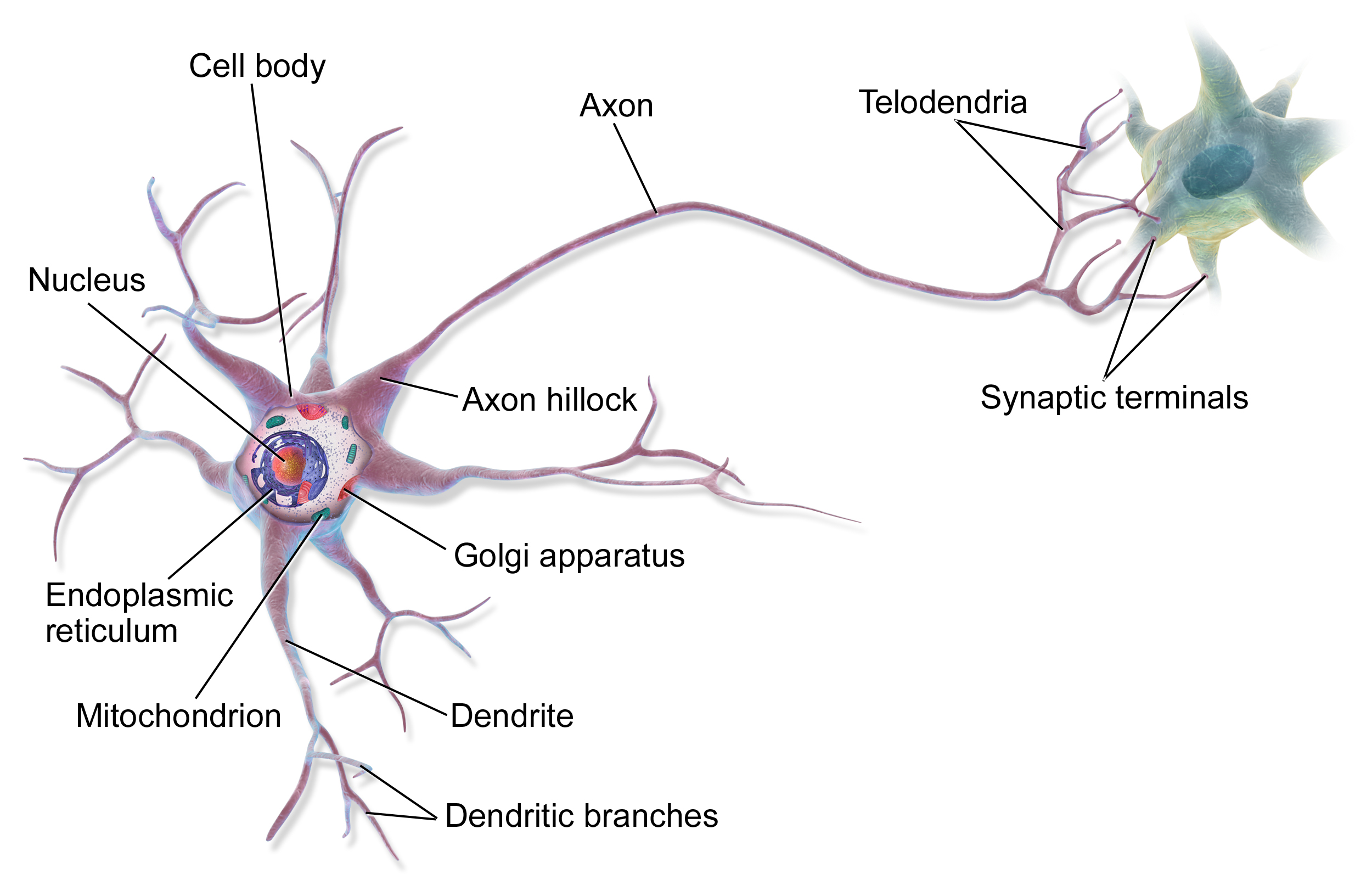
• Deep learning is a sub branch of machine learning, where artificial neural networks form highly complex predictive models
• Aka artificial intelligence (think of self-driving cars and alike)

Input: \( O = H_{j} \cdot w_{j} + H_{j+1} \cdot w_{j+1} + H_{j+...} \cdot w_{j+...} + H_{m} \cdot w_{m} + B_{H} \cdot w_{m+1} = \sum_{j}^{m} H_{j} \cdot w_{j} + B_{H} \cdot w_{m+1} = \sum_{j}^{m+1} H_{j} \cdot w_{j} = \textbf{H} \cdot \textbf{w} \)
Output: \( S(O) = \frac{1}{1+e^{-O}} \)

Error: \( E = MSE(O,T) = \frac{1}{2} \left( o - t \right)^2 \)
Updates: \( \Delta w = - \epsilon \frac{\delta E}{\delta w} \) and \( \Delta v = - \epsilon \frac{\delta E}{\delta v} \), where \( \epsilon \) is the learning rate

• They can identify context dependence!
• I.e. the “meaning” of each variable depends not only on its observed value, but also on the context in which it was observed!

• 1940's: Neurophysiologist Warren McCulloch and mathematician Walter Pitts wrote a paper on how neurons might work
• 1975: First multilayered back propagated network developed by Paul Werbos
• 2015: François Chollet, a Google engineer, releases Keras, a high level Deep Learning API
• 2015: Google releases TensorFlow as open source software
• 2017: Google's TensorFlow team decides to support Keras in TensorFlow's core library
• 2018: On day 2 at rstudio::conf 2018 in San Diego, RStudio CEO J.J. Allaire gives his keynote talk on “Machine Learning with R and TensorFlow”, officially announcing, that henceforth Keras and TensorFlow will by fully available in R
• These are exciting times and we as data scientists are at the epicenter of all these developments

• TensorFlow is an open source software library for numerical computations written in C++ (I.e. not confined to ANNs)
• Originally developed by researchers and engineers working on the Google Brain team within Google's Machine Intelligence Research organization for the purposes of conducting machine learning and deep neural networks research
• The core TensorFlow API is written in Python
• Keras is a high-level neural networks API, written in Python running on top of TensorFlow (or CNTK or Theano)
• Keras was developed by by François Chollet with a focus on enabling fast experimentation “Being able to go from idea to result with the least possible delay is key to doing good research”
• The Keras R-package is written in R by François Chollet and JJ Allaire
• The Keras interface is a really nice high level vocabulary for doing deep learning that fits really well with the way R-users work and think
• JJ Allaire has stated that “I have my heart in getting Keras and TensorFlow to work really really well in Deep Learning in R and hook into the RStudio IDE”
• The Keras R API calls the Keras Python API, which calls the core Python TensorFlow API which calls the TensorFlow C++ library
• Granted, a bit complicated, but my experience so far is, that it works

Sources: keras.io, tensorflow.rstudio.com, github.com/tensorflow, keras.rstudio.com, Machine Learning with R and TensorFlow, TensorFlow and Keras in R - Josh Gordon meets with J.J. Allaire

• TensorFlow APIs
  • keras - Interface for neural networks, with a focus on enabling fast experimentation
  • tfestimators - Implementations of common model types such as regressors and classifiers
  • tensorflow - Low-level interface the TensorFlow computational graph
  • tfdatasets - Scalable input pipelines for TensorFlow models
• Supporting tools
  • tfruns - Track, visualise and manage TensorFlow training runs and experiments
  • tfdeploy - Tools designed to make exporting and serving TensorFlow models straightforward
  • cloudml - R interface to Google Cloud Machine Learning Engine

Source: Machine Learning with R and TensorFlow 32:27

Using Hadley Wickham's devtools, it is straightforward to install both keras and TensorFlow:

install.packages('devtools')
devtools::install_github("rstudio/keras")
library("keras")
install_keras()

Hereafter all we will need to do, is run

library("keras")

That's it! Now we're ready to do deep learning in R!

Here is an illustration of the model we will be building with 35 parameters, i.e. \( (n_{features} + 1) \cdot m_{hidden} + (m_{hidden} + 1) \cdot l_{output} \)

We start with slightly wrangling the iris data set by renaming and scaling the features and converting character labels to numeric:

nn_dat = iris %>% as_tibble %>%
  mutate(sepal_l_feat = scale(Sepal.Length),
         sepal_w_feat = scale(Sepal.Width),
         petal_l_feat = scale(Petal.Length),
         petal_w_feat = scale(Petal.Width),          
         class_num    = as.numeric(Species) - 1, # factor, so = 0, 1, 2
         class_label  = Species) %>%
  select(contains("feat"), class_num, class_label)
nn_dat

# A tibble: 150 x 6
   sepal_l_feat sepal_w_feat petal_l_feat petal_w_feat class_num
          <dbl>        <dbl>        <dbl>        <dbl>     <dbl>
 1       -0.898       1.02          -1.34        -1.31        0.
 2       -1.14       -0.132         -1.34        -1.31        0.
 3       -1.38        0.327         -1.39        -1.31        0.
 4       -1.50        0.0979        -1.28        -1.31        0.
 5       -1.02        1.25          -1.34        -1.31        0.
 6       -0.535       1.93          -1.17        -1.05        0.
 7       -1.50        0.786         -1.34        -1.18        0.
 8       -1.02        0.786         -1.28        -1.31        0.
 9       -1.74       -0.361         -1.34        -1.31        0.
10       -1.14        0.0979        -1.28        -1.44        0.
# ... with 140 more rows, and 1 more variable: class_label <fct>

Here, we use scaling such that the mean of each feature is 0 and the standard deviation is 1

Then, we split the iris data into a training and a test data set, setting aside 20% of the data for left out data partition, to be used for final performance evaluation:

test_f = 0.20
nn_dat = nn_dat %>%
  mutate(partition = sample(c('train','test'), nrow(.), replace = TRUE, prob = c(1 - test_f, test_f)))

Based on the partition, we can now create training and test data, where x is a matrix and y is the one-hot encoding of the category

x_train = nn_dat %>% filter(partition == 'train') %>% select(contains("feat")) %>% as.matrix
y_train = nn_dat %>% filter(partition == 'train') %>% pull(class_num)          %>% to_categorical
x_test  = nn_dat %>% filter(partition == 'test')  %>% select(contains("feat")) %>% as.matrix
y_test  = nn_dat %>% filter(partition == 'test')  %>% pull(class_num)          %>% to_categorical

Thereby yielding

x_train %>% head(3)

     sepal_l_feat sepal_w_feat petal_l_feat petal_w_feat
[1,]   -0.8976739   1.01560199    -1.335752    -1.311052
[2,]   -1.5014904   0.09788935    -1.279104    -1.311052
[3,]   -1.0184372   0.78617383    -1.279104    -1.311052

y_train %>% head(3)

     [,1] [,2] [,3]
[1,]    1    0    0
[2,]    1    0    0
[3,]    1    0    0

With the data in place, we now set the architecture of our artificical neural network:

model = keras_model_sequential()
model %>% 
  layer_dense(units = 4, activation = 'sigmoid', input_shape = 4) %>% 
  layer_dense(units = 3, activation = 'softmax')

compile our model:

model %>% compile(
  loss      = 'categorical_crossentropy',
  optimizer = optimizer_rmsprop(),
  metrics   = c('accuracy')
)

and train our classifier

history = model %>% fit(
  x = x_train, y = y_train,
  epochs           = 200,
  batch_size       = 20,
  validation_split = 0,
  view_metrics     = FALSE,
  verbose = 0
)

The fit() function returns a history object, which we can plot like so

plot(history)

We can use the evaluate() function, to get the loss and accuracy metrics from the model

perf = model %>% evaluate(x_test, y_test)
print(perf)

$loss
[1] 0.3366045

$acc
[1] 0.972973

We can use the predict() and predict_classes() function for predicting soft and hard classifications respectively:

model %>% predict(x_test) %>% head

          [,1]       [,2]        [,3]
[1,] 0.8970004 0.09539866 0.007600991
[2,] 0.9257328 0.06898528 0.005281978
[3,] 0.9348749 0.06047851 0.004646669
[4,] 0.9333495 0.06154421 0.005106285
[5,] 0.9334606 0.06181232 0.004727044
[6,] 0.9097174 0.08376918 0.006513394

model %>% predict_classes(x_test) %>% head

[1] 0 0 0 0 0 0

…and finally we can visualise the confusion matrix based on the original 20% left out test data

• Using a bit of scraping, we can get data on all apartments sold in the regular market on Oesterbro since 2015

price_dat %>% dim

[1] 2667   12

price_dat %>% select(1:6) %>% head(3)

# A tibble: 3 x 6
  street        street_num floor_num date_of_sale quarter_of_sale rooms
  <chr>              <int>     <int> <date>                 <dbl> <int>
1 Østerbrogade          92         1 2018-02-27             2018.     3
2 Amerika Plads         36         2 2015-02-20             2015.     4
3 Amerika Plads         36         3 2015-08-06             2015.     4

price_dat %>% select(7:12) %>% head(3)

# A tibble: 3 x 6
    sqm    price sqm_price year_of_build   lon   lat
  <int>    <dbl>     <dbl>         <int> <dbl> <dbl>
1   136 7350000.    54044.          1904  12.6  55.7
2   103 3100000.    30097.          2008  12.6  55.7
3   103 3100000.    30097.          2008  12.6  55.7

• 2,667 observations of 12 variables (lon and lat are the longitude and latitude geocodes for the apartment address)

• The aim is to create a classifier for predicting the sales 'price class' of a given apartment
• First we will need to define the 'price class' of a given apartment
• We will create 3 price classes using the final sale price of the apartment:
  • \( class_0: z_{price} < -.5 \)
  • \( class_1: -.5 \leq z_{price} \leq .5 \)
  • \( class_2: .5 < z_{price} \)
• Where \( z_{price} \) is the scaled sales price of an apartment
• The set boundaries correspond roughly to dividing the probability density of a standard Gaussian in 3 equal parts

z_lim = 0.5
price_dat = price_dat %>%
  mutate(z_price = price %>% scale %>% as.numeric,
         price_class = ifelse( z_price < -z_lim, 0, ifelse( z_price < z_lim, 1, 2)))

• Thusly
  • \( class_0 \) apartments were sold for less than \( .5 \) standard deviations below the mean
  • \( class_1 \) apartments were sold for \( .5 \) standard deviations around the mean
  • \( class_2 \) apartments were sold for more than \( .5 \) standard deviations above the mean

• 7 features are selected: floor_num, quarter_of_sale, rooms, sqm, year_of_build, lon and lat
• 1 Output variable with 3 classes: price_class

price_dat_features = price_dat %>%
  select(floor_num, quarter_of_sale, rooms, sqm, year_of_build, lon, lat, price_class)
price_dat_features

# A tibble: 2,667 x 8
   floor_num quarter_of_sale rooms   sqm year_of_build   lon   lat
       <int>           <dbl> <int> <int>         <int> <dbl> <dbl>
 1         1           2018.     3   136          1904  12.6  55.7
 2         2           2015.     4   103          2008  12.6  55.7
 3         3           2015.     4   103          2008  12.6  55.7
 4         4           2015.     4   139          2008  12.6  55.7
 5         3           2016.     4   124          2008  12.6  55.7
 6         2           2017.     3    88          2005  12.6  55.7
 7         3           2017.     3    92          2005  12.6  55.7
 8         3           2017.     3    88          2005  12.6  55.7
 9         3           2015.     4    88          2005  12.6  55.7
10         0           2015.     3    96          2005  12.6  55.7
# ... with 2,657 more rows, and 1 more variable: price_class <dbl>

Now, we have the scaled feature data

nn_dat %>% head(3)

# A tibble: 3 x 8
  floor_num_feat quarter_of_sale_fe… rooms_feat sqm_feat year_of_build_fe…
           <dbl>               <dbl>      <dbl>    <dbl>             <dbl>
1         -0.675                1.73     0.0354    1.11             -0.736
2         -0.130               -1.45     0.829     0.308             1.90 
3          0.414               -1.24     0.829     0.308             1.90 
# ... with 3 more variables: lon_feat <dbl>, lat_feat <dbl>,
#   price_class <dbl>

Which we split the apartment data into a training and a test data set, setting aside 20% of the data for left out data partition, to be used for final performance evaluation:

test_f = 0.20
nn_dat = nn_dat %>%
  mutate(partition = sample(c('train','test'), nrow(.), replace = TRUE, prob = c(1 - test_f, test_f)))

Based on the partition, we can now create training and test data

x_train = nn_dat %>% filter(partition == 'train') %>% select(contains("feat")) %>% as.matrix
y_train = nn_dat %>% filter(partition == 'train') %>% pull(price_class)        %>% to_categorical
x_test  = nn_dat %>% filter(partition == 'test')  %>% select(contains("feat")) %>% as.matrix
y_test  = nn_dat %>% filter(partition == 'test')  %>% pull(price_class)        %>% to_categorical

With the data in place, we now set the architecture of our artificical neural network:

model = keras_model_sequential()
model %>% 
  layer_dense(units = 7, activation = 'sigmoid', input_shape = ncol(nn_dat)-2) %>% 
  layer_dense(units = 3, activation = 'softmax')

compile our model:

model %>% compile(
  loss      = 'categorical_crossentropy',
  optimizer = optimizer_rmsprop(),
  metrics   = c('accuracy')
)

and train our classifier

history = model %>% fit(
  x = x_train, y = y_train,
  epochs           = 100,
  batch_size       = 20,
  validation_split = 0.2,
  view_metrics     = FALSE,
  verbose = 0
)

We can use the evaluate() function, to get the loss and accuracy metrics from the model

perf = model %>% evaluate(x_test, y_test)
print(perf)

$loss
[1] 0.3757372

$acc
[1] 0.8513761

We can use the predict() and predict_classes() function for predicting soft and hard classifications respectively:

model %>% predict(x_test) %>% head

             [,1]      [,2]       [,3]
[1,] 0.0166475065 0.8399269 0.14342552
[2,] 0.0152409216 0.8286623 0.15609674
[3,] 0.0009843368 0.2008899 0.79812580
[4,] 0.0183639005 0.8461133 0.13552286
[5,] 0.0136891408 0.8010342 0.18527672
[6,] 0.0417256877 0.9254940 0.03278036

model %>% predict_classes(x_test) %>% head

[1] 1 1 2 1 1 1

…and finally we can visualise the confusion matrix based on the original 20% left out test data

• The peptide data set we will be working with consists of 7,920 positives and 7,920 negatives randomly split into 6 partitions:

pep_dat

# A tibble: 15,840 x 3
   peptide   binder partition
   <chr>      <int>     <int>
 1 LLTDAQRIV      0         1
 2 LMAFYLYEV      1         4
 3 VMSPITLPT      0         1
 4 SLHLTNCFV      0         5
 5 RQFTCMIAV      0         3
 6 FMNGHTHIA      1         2
 7 KINPYFSGA      0         3
 8 NIWLAIIEL      0         1
 9 KIMPYVAQF      0         2
10 AIWERACTI      0         3
# ... with 15,830 more rows

• The peptide variable, where the first observation is LLTDAQRIV is what we will use as input to our model
• Each letter denotes an amino acid, which is the basic building block our body, amazingly we only have 20 of these to build all the proteins of our body (think LEGO brick)
• Each amino acid is converted to a set of 21 numbers based on its bio-chemical properties
• Thusly, we have 189 input neurons (21 x 9)

Once again, we check the class balance

We will use partition 6 as independent test set and then do 5-fold cross validation on partitions 1-5

pep_dat_test_set = pep_dat %>% filter(partition == 6)
pep_dat = pep_dat %>% filter(partition != 6)

partitions  = pep_dat %>% count(partition) %>% pull(partition) # 1 2 3 4 5
data_splits = cross_fold_splits(partitions = partitions, print_splits = TRUE)

________________________________________________________________________________
Based on (1, 2, 3, 4, 5), the following 20 splits were created:
________________________________________________________________________________
Test partition = 1, Validation partition = 2, Training partitions = 3, 4, 5
Test partition = 1, Validation partition = 3, Training partitions = 2, 4, 5
Test partition = 1, Validation partition = 4, Training partitions = 2, 3, 5
Test partition = 1, Validation partition = 5, Training partitions = 2, 3, 4
Test partition = 2, Validation partition = 1, Training partitions = 3, 4, 5
Test partition = 2, Validation partition = 3, Training partitions = 1, 4, 5
Test partition = 2, Validation partition = 4, Training partitions = 1, 3, 5
Test partition = 2, Validation partition = 5, Training partitions = 1, 3, 4
Test partition = 3, Validation partition = 1, Training partitions = 2, 4, 5
Test partition = 3, Validation partition = 2, Training partitions = 1, 4, 5
Test partition = 3, Validation partition = 4, Training partitions = 1, 2, 5
Test partition = 3, Validation partition = 5, Training partitions = 1, 2, 4
Test partition = 4, Validation partition = 1, Training partitions = 2, 3, 5
Test partition = 4, Validation partition = 2, Training partitions = 1, 3, 5
Test partition = 4, Validation partition = 3, Training partitions = 1, 2, 5
Test partition = 4, Validation partition = 5, Training partitions = 1, 2, 3
Test partition = 5, Validation partition = 1, Training partitions = 2, 3, 4
Test partition = 5, Validation partition = 2, Training partitions = 1, 3, 4
Test partition = 5, Validation partition = 3, Training partitions = 1, 2, 4
Test partition = 5, Validation partition = 4, Training partitions = 1, 2, 3
________________________________________________________________________________

Set hyper parameters

model_activation    = "sigmoid"
model_learning_rate = 0.0001
model_optimizer     = optimizer_adam(lr = model_learning_rate)
model_loss          = 'mean_squared_error'
model_metrics       = 'mean_squared_error'
model_epochs        = 10
model_batch_size    = 20
model_layer_IN_n    = 189 # 9 amino acids x 21 enc values
model_layer_H1_n    = 189
model_layer_H2_n    = 90
model_layer_H3_n    = 45
model_layer_OUT_n   = 1

Set architecture

model = keras_model_sequential() %>% 
  layer_dense(units = model_layer_H1_n,  activation = model_activation, input_shape = model_layer_IN_n) %>% 
  layer_dense(units = model_layer_H2_n,  activation = model_activation) %>%
  layer_dense(units = model_layer_H3_n,  activation = model_activation) %>%
  layer_dense(units = model_layer_OUT_n, activation = model_activation)

Compiling the model

model %>% compile(loss = model_loss, optimizer = model_optimizer, metrics = model_metrics)

Note! The 20 splits result in our final model consisting of 20 models, each of which have 57,151 parameters. Together they form an ensembl of roughly 1,15 million parameters!

meta_data = list()
model_dir = 'models/'
for( mdl_i in names(data_splits) ){
  # Set partitions
  test_partition       = data_splits[[mdl_i]]$test_partition
  validation_partition = data_splits[[mdl_i]]$validation_partition
  training_partitions  = data_splits[[mdl_i]]$training_partitions

  # Set model file
  mdl_file = str_c(model_dir, mdl_i, ".hdf5")

  # Set callbacks used for early stopping
  callbacks_list = list( callback_early_stopping(monitor = "mean_squared_error", patience = 10),
                         callback_model_checkpoint(filepath = mdl_file, monitor = "val_loss",
                                                   save_best_only = TRUE) )
  # Extract and encode current training data
  pep_dat_training = pep_dat %>% filter(partition %in% training_partitions)
  x_train          = pep_dat_training %>% pull(peptide) %>% pep_encode_bl50 %>%
    array_reshape(c(dim(.)[1], dim(.)[2] * dim(.)[3]))
  y_train          = pep_dat_training %>% pull(binder) %>% array

  # Extract and encode current validation data
  pep_dat_validation = pep_dat %>% filter(partition %in% validation_partition)
  x_validation       = pep_dat_validation %>% pull(peptide) %>% pep_encode_bl50 %>%
    array_reshape(c(dim(.)[1], dim(.)[2] * dim(.)[3]))
  y_validation       = pep_dat_validation %>% pull(binder) %>% array

  # Do training
  history = model %>% fit(x = x_train, y = y_train, batch_size = model_batch_size, epochs = model_epochs,
                          callbacks = callbacks_list, validation_data = list(x_validation, y_validation))
  # Save meta data
  meta_data[[mdl_i]] = list(); meta_data[[mdl_i]]$mdl_file = mdl_file ; meta_data[[mdl_i]]$history = history
}

For each of the 20 models, we can now add predictions on the corresponding test set

for( mdl_id in names(meta_data) ){

  # Load current model  
  mdl = load_model_hdf5(filepath = meta_data[[mdl_id]]$mdl_file)
  meta_data[[mdl_id]]$model = mdl

  # Do prediction. Note how prediction are ONLY made for data points from the
  # test partition of the current model!
  pred_id = str_c('pred_', mdl_id)
  pep_dat = pep_dat %>% 
    mutate(!!pred_id := ifelse( partition == data_splits[[mdl_id]]$test_partition,
      pep_predict(peptide = peptide, model = mdl), NA))

}
# Calculate mean predictions
pep_dat = pep_dat %>% mutate(pred_model_mean = select(., contains('pred_')) %>% rowMeans(na.rm = TRUE))

pep_dat

# A tibble: 13,139 x 24
   peptide   binder partition pred_model_01 pred_model_02 pred_model_03
   <chr>      <int>     <int>         <dbl>         <dbl>         <dbl>
 1 LLTDAQRIV      0         1         0.528        0.125         0.0611
 2 LMAFYLYEV      1         4        NA           NA            NA     
 3 VMSPITLPT      0         1         0.231        0.0582        0.0256
 4 SLHLTNCFV      0         5        NA           NA            NA     
 5 RQFTCMIAV      0         3        NA           NA            NA     
 6 FMNGHTHIA      1         2        NA           NA            NA     
 7 KINPYFSGA      0         3        NA           NA            NA     
 8 NIWLAIIEL      0         1         0.334        0.269         0.534 
 9 KIMPYVAQF      0         2        NA           NA            NA     
10 AIWERACTI      0         3        NA           NA            NA     
# ... with 13,129 more rows, and 18 more variables: pred_model_04 <dbl>,
#   pred_model_05 <dbl>, pred_model_06 <dbl>, pred_model_07 <dbl>,
#   pred_model_08 <dbl>, pred_model_09 <dbl>, pred_model_10 <dbl>,
#   pred_model_11 <dbl>, pred_model_12 <dbl>, pred_model_13 <dbl>,
#   pred_model_14 <dbl>, pred_model_15 <dbl>, pred_model_16 <dbl>,
#   pred_model_17 <dbl>, pred_model_18 <dbl>, pred_model_19 <dbl>,
#   pred_model_20 <dbl>, pred_model_mean <dbl>

Only allow each model to predict on the unseen test partition

• Despite us only running the training for 10 epochs, the MSE decreases very rapidly!

• The area under the Receiver Operator Characterstics curve (the ROC curve) is the so called AUC value.
• If \( AUC = 1 \), then you have a perfect predictor, if \( AUC = 0.5 \), then you have a random predictor

Receiver Operator Characterstics curve

• For this set, we make 20 predictions for each \( x \) and assign the mean as the final prediction \( \hat{y} \)

Receiver Operator Characterstics curve

• With relatively little effort, we created a high performing ensembl model consisting of 1 input layer, 3 hidden layers and 1 output layer comprising a total of roughly 1,15 million parameters

((model_layer_IN_n + 1) * model_layer_H1_n + (model_layer_H1_n + 1) * model_layer_H2_n + (model_layer_H2_n + 1) * model_layer_H3_n + (model_layer_H3_n + 1) * model_layer_OUT_n) * 20

[1] 1143020

• The model obtained a performance of \( AUC = 0.984 \) on the overall model using 5-fold cross validation and \( AUC = 0.984 \) on the left out test set (partition 6)

• Be sure, that you “need” Deep Learning

  • Create a base learner using a simple approach, e.g. linear- or logistic regression model
  • Up the complexicity with e.g. a random forest model
  • Do a simple neural network, e.g. 1 input, 1 hidden and 1 output
  • Go full deep learning
  • Record the performance in each of the steps
  • If you max out using a logistic regression, then proceed no further

• Be aware that what you gain in performance, you may loose in model interpretability

• Be very careful with overfitting, a predictive model only works, if it can actually extrapolate on unseen data

• Check your data and partitions prior to modelling, sparsity, order, balance, etc.

• Naturally, deployment is really important as well!
• Now you spend all that time building your absolutely amazing deep learning model and now its time to put it to the test!
• Traditionally, with R when you do modelling and then if you want to deploy the model, you have to bring the R runtime along with you and that can be a challenge
• With the design of TensorFlow, you are writing a program, but that program is creating a graph and that graph is executed by a C++ runtime
• Therefore, deploying a model does not require, that you bring along R or Python runtimes in the deployment
• The tfdeploy package serialises the saved models, so you can put REST interfaces on top of models or get models brought into javascript using the library keras.js, which lets you take a keras model and run it directly in the browser
• With TensorFlow you can author models in R using the Keras interface and then deploy them straight into a browser
• This really brings together the best of two worlds: R is phenomenal for exploratory data analysis, training and authoring models and then you can deploy using languages well suited for deployment, e.g. javascript
• R users who want to put their models in production, now have a really straight forward way to do that
• Go to tensorflow.rstudio.com to get started!

Source: TensorFlow and Keras in R - Josh Gordon meets with J.J. Allaire

• Books

  • Deep Learning for R by Francois Chollet and J. J. Allaire
  • Free yet awesome book: R for Data Science by Garrett Grolemund and Hadley Wickham

• Coursera Deep Learning courses deeplearning.ai

• Meetup: CopenhagenR - useR Group

• tensorflow.rstudio.com

• keras.rstudio.com

• tensorflow.rstudio.com/learn

• Professor Morten Nielsen for allowing me to tab into his 25+ years of experience in using artificial neural networks for modeling biological systems
• Postdoctoral Researcher Vanessa Jurtz, with whom I collaborate on the netTCR project, part of which I prensented here today
• Professor Sine Reker Hadrup for generating data for me to play with
• The Independent Research Fund Denmark for paying my salery
• And then of course the organisers for giving me this oppertunity to talk about my research
• And should you be curious… Yes, I made this presentation in R

• TensorFlow for R is extremely powerful and flexible and allows you to create and deploy complex models in a relatively simple fashion
• Model building ends up being not about the code, but about mapping your problem and the data and the tools you have together to get a good solution
• The hard part about deep learning is not generally writing the code, the hard part is figuring out what sort of model to build, i.e. architecture and hyper paremeters, that's where all the time is spend!

Source: TensorFlow and Keras in R - Josh Gordon meets with J.J. Allaire