CAP 5610 Assignment#3 Danilo Martinez
Method A: . For each person, construct a subspace by PCA. . Given a test face, map it into these subspaces, and assign the face to the subspace with the minimal distance (reconstruction error as in objective function) Method B: . For all faces independent of people, construct a subspace by PCA . Using the reconstruction coefficients as a feature vector for each face . Applying existing classification algorithms (KNN, naive Bayes) . Will naive Bayes work this time?
Machine Problem 3 . Applying PCA to MNIST digital recognition . First, apply PCA (method B) to get a lower-dimensional feature representation . Choose the dimensionality of subspace for PCA . Each eigenvalue represents an energy component . Rank dimensions by their eigenvalues and preserve the top 95% energy . Use KNN in MP1 to the features obtained by PCA, report the performance . Repeat three protocols in MP1 to tune K . Repeat Naive Bayes in MP2 . This time, you do not need to tune ????; just use MLE instead
. Bonus credits (5 bonus points added to final score, submit in a separate report) . apply PCA (method A) to classify digit images. . Plot the obtained eigenvectors obtained by PCA (method A + method B)
One of the most commonly faced problems while dealing
with data analytics problem such as recommendation engines, text analytics is
high-dimensional and sparse data. At many times, we face a situation where we
have a large set of features and fewer data points, or we have data with very
high feature vectors. In such scenarios, fitting a model to the dataset,
results in lower predictive power of the model. This scenario is often termed
as the curse of dimensionality. In general, adding more data points or
decreasing the feature space, also known as dimensionality reduction, often
reduces the effects of the curse of dimensionality.
Principal Component Analysis, or PCA, is a useful statistical method that has
found application in a variety of fields and is a common technique for finding
patterns in data of high dimension. In simple words, principal component
analysis is a method of extracting important variables (in form of components)
from a large set of variables available in a data set. It extracts low
dimensional set of features from a high dimensional data set with a motive to
capture as much information as possible. With fewer variables, visualization
also becomes much more meaningful. PCA is more useful when dealing with 3 or
higher dimensional data. It is always performed on a symmetric correlation or
covariance matrix. This means the matrix should be numeric and have
standardized data. When faced with a large set of correlated variables,
principal components allow us to summarize this set with a smaller number of
representative variables that collectively explain most of the variability in
the original set. PCA is an unsupervised approach, since it involves only a set
of features X1,X2, . . . , Xp, and no associated response Y . Apart from
producing derived variables for use in supervised learning problems, PCA also
serves as a tool for data visualization (visualization of the observations or
visualization of the variables). PCA finds a low-dimensional representation of
a data set that contains as much as possible of the variation. The idea is that
each of the n observations lives in p-dimensional space, but not all of these
dimensions are equally interesting. PCA seeks a small number of dimensions that
are as interesting as possible, where the concept of interesting is measured by
the amount that the observations vary along each dimension. Each of the
dimensions found by PCA is a linear combination of the p features.
Mathematically speaking, PCA is a linear orthogonal transformation that
transforms the data to a new coordinate system such that the greatest variance
by any projection of the data comes to lie on the first coordinate (called the
first principal component), the second greatest variance on the second
coordinate, and so on. The algorithm when applied linearly transforms
m-dimensional input space to n-dimensional (n < m) output space, with the
objective to minimize the amount of information/variance lost by discarding
(m-n) dimensions. PCA allows us to discard the variables/features that have
less variance. Technically speaking, PCA uses orthogonal projection of highly
correlated variables to a set of values of linearly uncorrelated variables
called principal components. The number of principal components is less than or
equal to the number of original variables. This linear transformation is
defined in such a way that the first principal component has the largest
possible variance. It accounts for as much of the variability in the data as
possible by considering highly correlated features. Each succeeding component
in turn has the highest variance using the features that are less correlated
with the first principal component and that are orthogonal to the preceding
component.
There's no way to map high-dimensional data into low dimensions and preserve all the structure. So, an approach must make trade-offs, sacrificing one property to preserve another. PCA tries to preserve linear structure. A principal component is a normalized linear combination of the original predictors in a data set. The first principal component is a linear combination of original predictor variables which captures the maximum variance in the data set. It determines the direction of highest variability in the data. Larger the variability captured in first component, larger the information captured by component. No other component can have variability higher than first principal component.
The first principal component results in a line which is closest to the data minimizing the sum of squared distance between a data point and the line. The second principal component is also a linear combination of original predictors which captures the remaining variance in the data set and is uncorrelated with the first principal component. If the two components are uncorrelated, their directions should be orthogonal. This suggests the correlation between these components is zero. All succeeding principal component follows a similar concept. They capture the remaining variation without being correlated with the previous component. The directions of these components are identified in an unsupervised way so the response variable(Y) is not used to determine the component direction. Therefore, it is an unsupervised approach. The principal components are supplied with normalized version of original predictors because the original predictors may have different scales. Performing PCA on un-normalized variables will lead to insanely large loadings for variables with high variance. In turn, this will lead to dependence of a principal component on the variable with high variance, and this is undesirable. As far as K neighrest neighbor: In protocol 1, as we increase K, one can see that the error drops and then increases , best K = 3. In protocol 2, we as we increase k, one can see that the error increases, and the variability also increases. Best K = 1 The ideal K that was generated in cross validation was K = 3, which is actually the lowest point in protocol 1 and near the lowest point in protocol 2 prior to the variability. Cross Validation 10 Fold had the lowest variance at K = 3. For KNN using PCA, we would chose K = 3 as the preferred K with Cross Validation. As far as Naive Bayes Classifier: Protocol 2 produced the lowest error (.1548218). Therefore, the validation approach for Naive Bayes is the best.
Overall, using PCA improved performance for both KNN and Bayes. I must disclose that in assignment 1, I sampled observations for KNN because of the time it was taking to process. In this assignment, I did not sample and used the entire training, validation, and test sets. They processed much quicker thanks to the PCA processing of the data. Between both naive Bayes and KNN, KNN Cross Validation with K = 3 is the best choice.
Every MNIST data point, every image, can be thought of as an array of numbers describing how dark each pixel is. Since each image has 28 by 28 pixels, we get a 28x28 array. We can flatten each array into a 28???28=784 dimensional vector. Each component of the vector is a value between zero and one describing the intensity of the pixel. Thus, we generally think of MNIST as being a collection of 784-dimensional vectors. Not all vectors in this 784-dimensional space are MNIST digits. Using 95% of the variation, and maintaining 154 principal components when performing PCA, is the key to the improvement in accuracy.
Setting up data and performing Principal Component Analysis.
#Loading
necessary Libraries
library(class)
library(caret)
library(mnist)
library(doParallel)
# Setting up parallel
processing.
cl <-makeCluster(detectCores())
registerDoParallel(cl)
#Fetching the data set
from the MNIST website
mnist <- download_mnist()
#Extracting the the first
60k observations
inTrain =head(mnist, 60000)
#Removing Unnecessary
files
rm(mnist)
#Creating matrices for Xs
and Y
responseY <- as.factor(inTrain[,dim(inTrain)[2]])
predictorX <- as.matrix(inTrain[,1:(dim(inTrain)[2]-1)])
#Removing Unnecessary
files
rm(inTrain)
#Performing Principal
Componenet Analysis
pca <- prcomp(predictorX,cor=F)
cumvar<-cumsum(pca$sdev^2 / sum(pca$sdev^2))
#Selecting the PC's that
maintain 95% of the variation
pc.index<-min(which(cumvar>0.95))
pc.comp <- pca$scores
pc.comp1 <- -1*pc.comp[,1]
#Combining the PC's for
predictions in models
X = cbind(pc.comp1,-1*pca$x[,2:pc.index])
#Displaying the total
number of PC's used
print("The total number of
principal components used is")
## [1] "The total number of principal components used is"
print(pc.index)
## [1] 154
#Removing
Unnecessary files
rm(predictorX)
rm(pca)
rm(cumvar)
rm(pc.index)
rm(pc.comp)
rm(pc.comp1)
RESULTS: Training set 50,000, Test set 10,000, K = 1 through 15.
#Dividing
50k for training and 10k for testing
trainIndex = createDataPartition(responseY, p=0.833245, list=FALSE)
#Setting up the testing
index for later dividing dataset
testindex=-trainIndex
#Setting up data for test
errors
test.error = c()
#Creating model using K
Nearest neighbor
for (i in seq(1, 15, 2))
{
cat("Processing KNN using K =
", i, "\n", sep = "")
model<- knn(train=X[trainIndex,], test=X[-trainIndex,], cl=responseY[trainIndex],k=i, prob=F)
test.error[i]<-sum(model!=responseY[-trainIndex])/length(responseY[-trainIndex])
print(test.error[i])
}
##
Processing KNN using K = 1
## [1] 0.0301
## Processing KNN using
K = 3
## [1] 0.0289
## Processing KNN using
K = 5
## [1] 0.0304
## Processing KNN using
K = 7
## [1] 0.0324
## Processing KNN using
K = 9
## [1] 0.0335
## Processing KNN using
K = 11
## [1] 0.0354
## Processing KNN using
K = 13
## [1] 0.0367
## Processing KNN using
K = 15
## [1] 0.0399
#Plotting
test errors
plot(test.error,col='red', type = 'b', ylab = "K Neighbors",main = "Test Errors",ylim = c(0,0.1))

The preferred for protocol 1 is K = 3.
2nd Test Protocol Training set 40,000, Validation set 10,000, Test set 10,000, K = 1 through 15.
#Setting
up data for test errors
test.error = c()
#Dividing data with
training having 40k, validation set having 10k, and testing having 10k.
trainIndex = createDataPartition(responseY, p=0.666565, list=FALSE)
#Creating model using K
Nearest neighbor
for (i in seq(1, 15, 2))
{
cat("Processing KNN using K =
", i, "\n", sep = "")
model<- knn(train=X[trainIndex,], test=X[-trainIndex:testindex-1,], cl=responseY[trainIndex],k=i, prob=F)
test.error[i]<-sum(model!=responseY[-trainIndex:testindex-1])/length(responseY[-trainIndex:testindex-1])
print(test.error[i])
}
## Processing
KNN using K = 1
## [1] 0.009700162
## Processing KNN using
K = 3
## [1] 0.01941699
## Processing KNN using
K = 5
## [1] 0.02406707
## Processing KNN using
K = 7
## [1] 0.02658378
## Processing KNN using
K = 9
## [1] 0.02953383
## Processing KNN using
K = 11
## [1] 0.03230054
## Processing KNN using
K = 13
## [1] 0.03405057
## Processing KNN using
K = 15
## [1] 0.03533392
#Plotting
test errors
plot(test.error,col='red', type = 'b', ylab = "K Neighbors",main = "Test Errors",ylim = c(0,0.1))

Applying the model picked from validation set, to test set using K = 1.
#Creating model using K Nearest
neighbor
cat("Processing KNN using K =
", 1, "\n", sep = "")
## Processing KNN using K = 1
model<- knn(train=X[trainIndex,], test=X[-trainIndex:testindex-1,], cl=responseY[trainIndex],k=1, prob=F)
test.error[1]<-sum(model!=responseY[-trainIndex:testindex-1])/length(responseY[-trainIndex:testindex-1])
print(test.error[1])
## [1] 0.009700162
3rd Protocol 5-fold cross-validation and 10-fold cross validation (average and standard deviation)
library(e1071)
#Full Data set can be
used for cross validation
for (i in seq(5, 10, 5))
{
cat("Processing KNN using Cross
Validation " ,i,"
Folds\n",sep = "")
#Setting seed to produce same
results
set.seed(123)
knn.cross <- tune.knn(x = X, y = responseY, k =seq(1,5,2), tunecontrol=tune.control(sampling = "cross"), cross=i)
#Summarize the resampling
results set
plot(knn.cross)
summary(knn.cross)
}
## Processing KNN using Cross Validation 5 Folds
## Processing KNN using Cross Validation 10 Folds
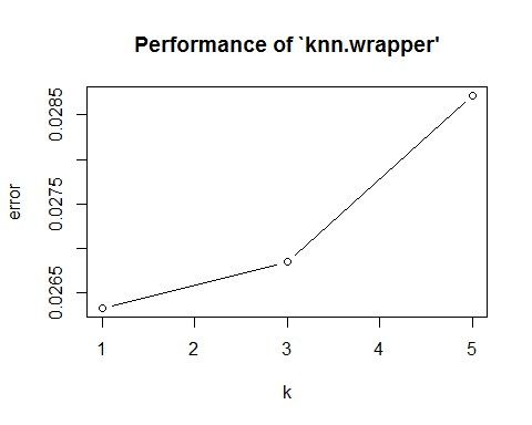
The 5 Fold cross validation approach has a lowest error at K = 1, while the 10 Fold validation approach has similar lower average errors at K =1 and K = 3. 10 Fold Validationhas has a lower variance at K = 3. The generated best K is K = 1, containing the ideal lowest error, but not by much. If we are interested in least amount of variability within our model and data, then we can choose the 10 Fold approach, with K = 3 in this case.
#Dividing
50k for training and 10k for testing
trainIndex = createDataPartition(responseY, p=0.833245, list=FALSE)
#Setting up the testing
index for later dividing dataset
testindex=-trainIndex
#Creating model using
Naive Bayes Classifier
cat("Processing Naive Bayes
Classifier 50k training, 10k testing.","\n",sep = "")
## Processing Naive Bayes Classifier 50k training, 10k testing.
nb_model<-
naiveBayes(X[trainIndex,],responseY[trainIndex])
results<-predict(nb_model,newdata=X[-trainIndex,],type=c("class"))
output <-confusionMatrix(results,responseY[-trainIndex])
print("Prior(Y) Maximum
Likelihood Estimate, Prevalence Detection & Maximum a Priori (Balanced
Accuracy)")
## [1] "Prior(Y) Maximum Likelihood Estimate, Prevalence Detection & Maximum a Priori (Balanced Accuracy)"
print(output$byClass)
##
Sensitivity Specificity Pos Pred Value Neg Pred Value Precision
## Class: 0
0.8946302 0.9799179 0.8298872 0.9883617 0.8298872
## Class: 1
0.9261566 0.9984227 0.9867299 0.9907211 0.9867299
## Class: 2
0.8459215 0.9522594 0.6614173 0.9824742 0.6614173
## Class: 3
0.8052838 0.9855202 0.8635887 0.9780038 0.8635887
## Class: 4
0.8018480 0.9873698 0.8726257 0.9788029 0.8726257
## Class: 5 0.8294574
0.9790041 0.7968085 0.9830022 0.7968085
## Class: 6
0.8955375 0.9946750 0.9484425 0.9886426 0.9484425
## Class: 7
0.8266284 0.9930773 0.9329730 0.9800551 0.9329730
## Class: 8
0.8482051 0.9860388 0.8677859 0.9836410 0.8677859
## Class: 9
0.8064516 0.9762433 0.7889546 0.9786334 0.7889546
##
Recall F1 Prevalence Detection Rate
## Class: 0 0.8946302
0.8610434 0.0987 0.0883
## Class: 1 0.9261566
0.9554842 0.1124 0.1041
## Class: 2 0.8459215
0.7423774 0.0993 0.0840
## Class: 3 0.8052838
0.8334177 0.1022 0.0823
## Class: 4 0.8018480
0.8357410 0.0974 0.0781
## Class: 5 0.8294574
0.8128052 0.0903 0.0749
## Class: 6 0.8955375
0.9212311 0.0986 0.0883
## Class: 7 0.8266284
0.8765871 0.1044 0.0863
## Class: 8 0.8482051
0.8578838 0.0975 0.0827
## Class: 9 0.8064516
0.7976072 0.0992 0.0800
## Detection
Prevalence Balanced Accuracy
## Class:
0 0.1064 0.9372740
## Class:
1 0.1055 0.9622896
## Class:
2 0.1270 0.8990904
## Class:
3 0.0953 0.8954020
## Class:
4 0.0895 0.8946089
## Class:
5 0.0940 0.9042307
## Class:
6 0.0931 0.9451062
## Class:
7 0.0925 0.9098528
## Class:
8 0.0953 0.9171220
## Class:
9 0.1014 0.8913475
print("Overall Error Rate")
## [1] "Overall Error Rate"
acc=output$overall['Accuracy']
print(1-as.numeric(acc))
## [1] 0.151
#Dividing
data with training having 40k, validation set having 10k, and testing having
10k.
trainIndex = createDataPartition(responseY, p=0.666565, list=FALSE)
#Creating model using
Naive Bayes Classifier
cat("Processing Naive Bayes
Classifier 40k training, 10k validation, and 10k testing.","\n",sep = "")
## Processing Naive Bayes Classifier 40k training, 10k validation, and 10k testing.
nb_model<-
naiveBayes(X[trainIndex,],responseY[trainIndex])
results<-predict(nb_model,newdata=X[-trainIndex:testindex-1,],type=c("class"))
output <-confusionMatrix(results,responseY[-trainIndex:testindex-1])
print("Prior(Y) Maximum
Likelihood Estimate, Prevalence Detection & Maximum a Priori (Balanced
Accuracy)")
## [1] "Prior(Y) Maximum Likelihood Estimate, Prevalence Detection & Maximum a Priori (Balanced Accuracy)"
print(output$byClass)
##
Sensitivity Specificity Pos Pred Value Neg Pred Value Precision
## Class: 0
0.8953056 0.9806202 0.8349606 0.9884434 0.8349606
## Class: 1
0.9247998 0.9975966 0.9798837 0.9905474 0.9798837
## Class: 2
0.8538100 0.9528506 0.6662737 0.9833664 0.6662737
## Class: 3
0.8101452 0.9809163 0.8285238 0.9784460 0.8285238
## Class: 4
0.8176994 0.9880902 0.8810402 0.9804863 0.8810402
## Class: 5
0.7976388 0.9788559 0.7893392 0.9798793 0.7893392
## Class: 6
0.8661710 0.9942679 0.9429728 0.9854847 0.9429728
## Class: 7
0.8260176 0.9932631 0.9346216 0.9799860 0.9346216
## Class: 8
0.8314818 0.9847640 0.8550088 0.9818446 0.8550088
## Class: 9
0.8166078 0.9771508 0.7973084 0.9797611 0.7973084
##
Recall F1 Prevalence Detection Rate
## Class: 0 0.8953056
0.8640808 0.09870165 0.08836814
## Class: 1 0.9247998
0.9515452 0.11236854 0.10391840
## Class: 2 0.8538100
0.7484735 0.09930166 0.08478475
## Class: 3 0.8101452
0.8192314 0.10218504 0.08278471
## Class: 4 0.8176994
0.8481889 0.09736829 0.07961799
## Class: 5 0.7976388
0.7934673 0.09035151 0.07206787
## Class: 6 0.8661710
0.9029417 0.09863498 0.08543476
## Class: 7 0.8260176
0.8769700 0.10441841 0.08625144
## Class: 8 0.8314818
0.8430812 0.09751829 0.08108468
## Class: 9 0.8166078
0.8068427 0.09915165 0.08096802
## Detection
Prevalence Balanced Accuracy
## Class: 0
0.10583510 0.9379629
## Class: 1
0.10605177 0.9611982
## Class: 2
0.12725212 0.9033303
## Class: 3
0.09991833 0.8955307
## Class: 4
0.09036817 0.9028948
## Class: 5
0.09130152 0.8882474
## Class: 6
0.09060151 0.9302194
## Class: 7
0.09228487 0.9096403
## Class: 8
0.09483491 0.9081229
## Class: 9
0.10155169 0.8968793
print("Overall Error Rate")
## [1] "Overall Error Rate"
acc=output$overall['Accuracy']
print(1-as.numeric(acc))
## [1] 0.1547192
#Dividing
50k for training and 10k for testing
trainIndex = createDataPartition(responseY, p=0.833245, list=FALSE)
for (i in seq(5, 10, 5))
{
#Creating model using
Naive Bayes Classifier
cat("Processing Naive Bayes
using Cross Validation " ,i,
" Folds\n",sep = "")
ctrl <- trainControl(method = "cv", number = i)
nb_model<- naiveBayes(X[trainIndex,],responseY[trainIndex],ctrl)
results<-predict(nb_model,newdata=X[-trainIndex,],type=c("class"))
output <-confusionMatrix(results,responseY[-trainIndex])
print("Prior(Y) Maximum
Likelihood Estimate, Prevalence Detection & Maximum a Priori (Balanced
Accuracy)")
print(output$byClass)
print("Overall Error Rate")
acc=output$overall['Accuracy']
print(1-as.numeric(acc))
cat("\n")
}
##
Processing Naive Bayes using Cross Validation 5 Folds
## [1] "Prior(Y)
Maximum Likelihood Estimate, Prevalence Detection & Maximum a Priori
(Balanced Accuracy)"
## Sensitivity
Specificity Pos Pred Value Neg Pred Value Precision
## Class: 0
0.9057751 0.9776989 0.8164384 0.9895564 0.8164384
## Class: 1
0.9208185 0.9966201 0.9718310 0.9900392 0.9718310
## Class: 2
0.8388721 0.9501499 0.6497660 0.9816472 0.6497660
## Class: 3
0.8013699 0.9770550 0.7990244 0.9773816 0.7990244
## Class: 4
0.8121150 0.9889209 0.8877666 0.9799100 0.8877666
## Class: 5
0.8017719 0.9793338 0.7938596 0.9803037 0.7938596
## Class: 6
0.8559838 0.9961172 0.9601820 0.9844315 0.9601820
## Class: 7
0.8247126 0.9938589 0.9399563 0.9798547 0.9399563
## Class: 8
0.8225641 0.9836011 0.8442105 0.9808840 0.8442105
## Class: 9 0.8094758
0.9797957 0.8152284 0.9790349 0.8152284
##
Recall F1 Prevalence Detection Rate
## Class: 0 0.9057751
0.8587896 0.0987 0.0894
## Class: 1 0.9208185
0.9456373 0.1124 0.1035
## Class: 2 0.8388721 0.7323077
0.0993 0.0833
## Class: 3 0.8013699
0.8001954 0.1022 0.0819
## Class: 4 0.8121150
0.8482574 0.0974 0.0791
## Class: 5 0.8017719
0.7977961 0.0903 0.0724
## Class: 6 0.8559838
0.9050938 0.0986 0.0844
## Class: 7 0.8247126
0.8785714 0.1044 0.0861
## Class: 8 0.8225641
0.8332468 0.0975 0.0802
## Class: 9 0.8094758
0.8123419 0.0992 0.0803
## Detection
Prevalence Balanced Accuracy
## Class: 0 0.1095
0.9417370
## Class:
1 0.1065 0.9587193
## Class:
2 0.1282 0.8945110
## Class:
3 0.1025 0.8892124
## Class:
4 0.0891 0.9005179
## Class: 5 0.0912
0.8905529
## Class:
6 0.0879 0.9260505
## Class:
7 0.0916 0.9092858
## Class:
8 0.0950 0.9030826
## Class:
9 0.0985 0.8946358
## [1] "Overall
Error Rate"
## [1] 0.1594
##
## Processing Naive
Bayes using Cross Validation 10 Folds
## [1] "Prior(Y)
Maximum Likelihood Estimate, Prevalence Detection & Maximum a Priori
(Balanced Accuracy)"
## Sensitivity
Specificity Pos Pred Value Neg Pred Value Precision
## Class: 0
0.9057751 0.9776989 0.8164384 0.9895564 0.8164384
## Class: 1
0.9208185 0.9966201 0.9718310 0.9900392 0.9718310
## Class: 2
0.8388721 0.9501499 0.6497660 0.9816472 0.6497660
## Class: 3 0.8013699
0.9770550 0.7990244 0.9773816 0.7990244
## Class: 4
0.8121150 0.9889209 0.8877666 0.9799100 0.8877666
## Class: 5
0.8017719 0.9793338 0.7938596 0.9803037 0.7938596
## Class: 6
0.8559838 0.9961172 0.9601820 0.9844315 0.9601820
## Class: 7
0.8247126 0.9938589 0.9399563 0.9798547 0.9399563
## Class: 8
0.8225641 0.9836011 0.8442105 0.9808840 0.8442105
## Class: 9
0.8094758 0.9797957 0.8152284 0.9790349 0.8152284
##
Recall F1 Prevalence Detection Rate
## Class: 0 0.9057751
0.8587896 0.0987 0.0894
## Class: 1 0.9208185
0.9456373 0.1124 0.1035
## Class: 2 0.8388721
0.7323077 0.0993 0.0833
## Class: 3 0.8013699 0.8001954
0.1022 0.0819
## Class: 4 0.8121150
0.8482574 0.0974 0.0791
## Class: 5 0.8017719
0.7977961 0.0903 0.0724
## Class: 6 0.8559838
0.9050938 0.0986 0.0844
## Class: 7 0.8247126
0.8785714 0.1044 0.0861
## Class: 8 0.8225641
0.8332468 0.0975 0.0802
## Class: 9 0.8094758
0.8123419 0.0992 0.0803
## Detection
Prevalence Balanced Accuracy
## Class:
0 0.1095 0.9417370
## Class:
1 0.1065 0.9587193
## Class:
2 0.1282 0.8945110
## Class:
3 0.1025 0.8892124
## Class:
4 0.0891 0.9005179
## Class:
5 0.0912 0.8905529
## Class:
6 0.0879 0.9260505
## Class:
7 0.0916 0.9092858
## Class:
8 0.0950 0.9030826
## Class:
9 0.0985 0.8946358
## [1] "Overall
Error Rate"
## [1] 0.1594
The 5 Fold cross validation and the 10 Fold validation
approaches have an equivalent average error, and interestingly enough, not a
huge difference from protocol 1 and protocol 2. Protocol 2, validation
approach, is the lowest (.1548218).
The generated best for Naive Bayes, containing the ideal lowest error, is the
validation approach.
www.quora.com ISLR texbook