- All objects in R have a class
- Classes can be combined
- Spatial class systems
Slides: github.com/ITSLeeds/R4TA
An introduction to classes
Common R classes
- Vectors
- Matrices
- Lists
- Data frames
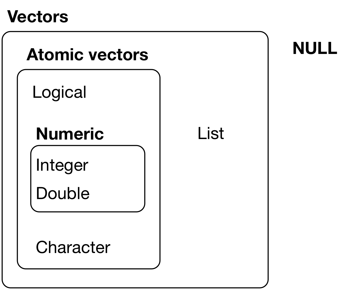
x = 1
class(x)
## [1] "numeric"
typeof(x)
## [1] "double"
dim(x)
## NULL
Vectors
Practical 1: Getting used to RStudio and R
- Open RStudio and have a look around
- Create a new project
- Create a new R Script: pass code to the console with
Ctl-Enter - Use R as a calculator: what is:
\[ \pi * 9.15^2 \]
- Explore each of the 'panes'
- Find and write down some useful shortcuts (
Alt-Shift-Kon Windows/Linux)
Basic R functions and behaviour
Functions and objects
In R:
- Everything that exists is an object
- Everything that happens is a function
x = 5
Functions
sin(x)
## [1] -0.9589243
exp(x)
## [1] 148.4132
sinx = sin(x)
Creating new functions
plus1 = function(x) {
  x + 1
}
plus1(x)
## [1] 6
R is vector based
x = c(1, 2, 5)
x
## [1] 1 2 5
x^2
## [1] 1 4 25
x + 2
## [1] 3 4 7
x + rev(x)
The classic programming way: verbose
x = c(1, 2, 5)
for(i in x){
  print(i^2)
}
## [1] 1
## [1] 4
## [1] 25
Creating a new vector based on x
for(i in 1:length(x)){
  if(i == 1) x2 = x[i]^2
  else x2 = c(x2, x[i]^2)
}
x2
## [1] 1 4 25
Data types
R has a hierarchy of data classes, tending to the lowest:
- Binary
- Integer (numeric)
- Double (numeric)
- Character
Examples of data types
a = TRUE
b = 1:5
c = pi
d = "Hello Leeds"
class(a)
class(b)
class(c)
class(d)
Data type switching
ab = c(a, b)
ab
## [1] 1 1 2 3 4 5
class(ab)
## [1] "integer"
Test on data types
class(c(a, b))
## [1] "integer"
class(c(a, c))
## [1] "numeric"
class(c(b, d))
## [1] "character"
Sequences
x = 1:5
y = 2:6
plot(x, y)

Sequences with seq
x = seq(1,2, by = 0.2)
length(x)
## [1] 6
x = seq(1, 2, length.out = 5)
length(x)
## [1] 5
- Challenge: create a list containing logical, character and numeric vectors
- What happens to the class if you unlist this list?
Challenges
- Complete all the code examples in 20.4
- Challenge: what are the outcomes of the following commands?:
x = 1:10
x[c(1, NA)]
x[2 * 3]
x[-2 * 3]
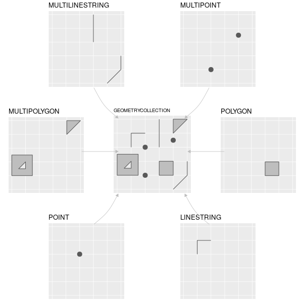
Spatial data classes
sf objects
sf is a package and class system for geographic data
library(sf)
## Linking to GEOS 3.5.1, GDAL 2.2.2, proj.4 4.9.2
Enables geographic data creation, e.g. with:
x = 1:9
y = x^2
xdf = data.frame(v1 = x, x = x, y = y)
xsf = st_as_sf(x = xdf, coords = c("x", "y"))
Types of sf object
What's in an sf object?
class(xsf)
## [1] "sf" "data.frame"
names(xsf)
## [1] "v1" "geometry"
xsf$geometry[1]
## Geometry set for 1 feature
## geometry type:  POINT
## dimension:      XY
## bbox:           xmin: 1 ymin: 1 xmax: 1 ymax: 1
## epsg (SRID):    NA
## proj4string:    NA
## POINT (1 1)
unclass(xsf$geometry[1][[1]])
## [1] 1 1
attributes(xsf$geometry[1][[1]])
## $class
## [1] "XY"    "POINT" "sfg"
Creating sf objects manually
- Not recommended!
(xy = st_point(c(5, 2))) # XY point
## POINT (5 2)
(xyg = st_sfc(xy))
## Geometry set for 1 feature
## geometry type:  POINT
## dimension:      XY
## bbox:           xmin: 5 ymin: 2 xmax: 5 ymax: 2
## epsg (SRID):    NA
## proj4string:    NA
## POINT (5 2)
(xysf = st_sf(xyg))
## Simple feature collection with 1 feature and 0 fields
## geometry type:  POINT
## dimension:      XY
## bbox:           xmin: 5 ymin: 2 xmax: 5 ymax: 2
## epsg (SRID):    NA
## proj4string:    NA
##           xyg
## 1 POINT (5 2)
Exercises
Talk about the pros and cons of vector data in your field of application with your neighbour: when would you be persuaded to use raster data?
Work through section 2.1 of Chapter 2, focussing on the code (not the text)
Complete the exercises 1:3 in Chapter 2
Bonus: work through section 20.4 in r4ds and complete the exercises in section 20.4.6