Strength of Concrete

Brian Kreis
April 24, 2018

Observational vs Designed Experiments

Obeservational Data Sets

  • Thus far this is what we have been working with, existing predictor data
  • Often comes in the form of a large comprehensive data set

Designed Experiments

  • Prefer a sequence of studies rather than one large data set
  • Involves planning, designing and analyzing an experiment
  • Here we will use predictive measures to identify ingredient proportions for further testing

Designed Experiments

  • Methods used to plan the exact values of predictors (factors)
  • Begin with a balanced design
  • Sequential Experimentation is used to determine important factors
  • Response Surface Experiments

Concrete

Concrete is integral for the infrastructure of industrial societies. Its strength and the optimal makeup to improve that strength have been widely studied. We will look at the various proportions of mixture ingredients to maximize compressive strength.

The ingredients of interest are cement, fly ash, blast furnace slag, water, superplasticizer, coarse & fine aggregate. All at a scale of kg/m3.
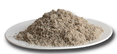
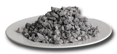
plot of chunk unnamed-chunk-1plot of chunk unnamed-chunk-1

A Quick Look at Each Variable

plot of chunk unnamed-chunk-2

plot of chunk unnamed-chunk-3

Predictor Plotted with Outcome

  • Age shows nonlinear relationship with compressive strength
  • Cement appears linear
  • Some high frequencies at specific values

plot of chunk unnamed-chunk-4

Predictors

The predictors will enter the model as a proportion of the total mixture

  • Built in dependency between the predictors
  • Pairwise correlations were not found to be large
  • Observations with duplicate measures have outcomes averaged

The Models

  • Linear regression, partial least squares, and the elastic net
  • Support vector machines (SVMs).
  • Neural network
  • MARS
  • Regression trees, model trees (with and without rules), and Cubist
  • Bagged and boosted regression trees & random forest models

  • Will use 10-fold cross validation

Parallel Processing

###For MAC:
#library(doMC)
#registerDoMC(cores = 2)

###For Windows
library(parallel)
library(doParallel)

cluster <- makeCluster(detectCores() - 1) # convention to leave 1 core for OS
registerDoParallel(cluster)
#caret package functions will now use multiple cores
#turn off parallel processing
stopCluster(cluster)
#resume use of the sequential backend
registerDoSEQ()

Time functions

Simple way to check speed improvements of code

library(tictoc)
tic(
Sys.sleep(3)
)
toc()
3 sec elapsed

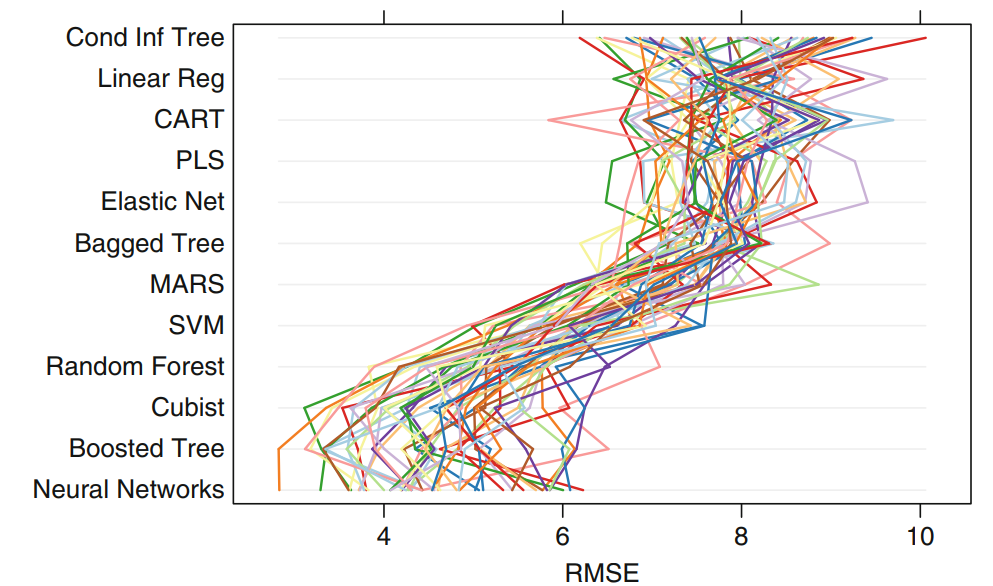
Results - RMSE

Parallel coordinate plot showing performance for each cross validation set
plot of chunk unnamed-chunk-7

Results - R2

Parallel coordinate plot showing performance for each cross validation set
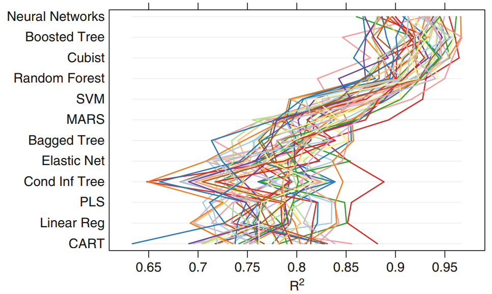
plot of chunk unnamed-chunk-8

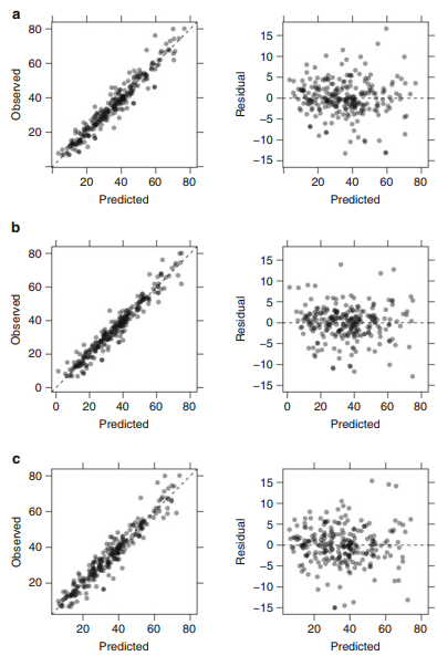
Top 3 Models - Based on RMSE

Neural Network - 4.2 RMSE (a)

  • 27 hidden units
  • Weight decay of 0.1

Boosted Tree - 3.9 RMSE (b)

  • Chose fast learning rate and deep trees

Cubist - 4.5 RMSE (c )

  • 100 committees
  • Predictions adjusted with 3 nearest neighbors

Optimizing Compressive Strength

Now that we know which models appear to be best at predicting, how do we find the improved mixtures?

A numerical search routine

  • Search seven dimensional space using direct methods
  • Two were used by the authors: Nelder Mead simplex method and simulated annealing
  • Simplex search method had the best results

Once we determine potential improved mixtures, further experiments will be needed

Optimizing Compressive Strength - 2

  • The search routines begin with intital starting values

  • For Nelder-Mead multiple starting places should be used and results compared

    • Used values with age 15 - 28 days to generate starting points
  • Values which are impractical or impossible are avoided by setting the amount

    • Water did not occur at a value of less than 5.1%, so this was set to a minimum of 5%

Search Results

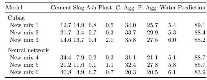
Predicted compressive strength and mixture composition compared to our highest values of 81.75, 79.99 and 78.8 in our training set:
PCA Plot
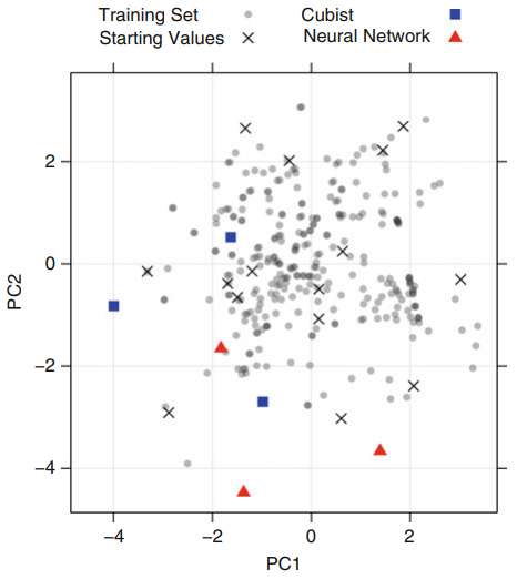
  • PCA plot shows the mixtures in 7 dimensional space using two components
  • Some of the top predicted models are near the edges of the prediction space
    • Could represent inaccuracy due to extrapolation
    • Experiment needed

Multiparameter Optimization

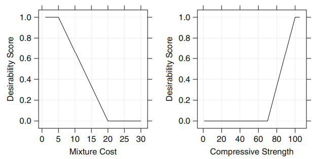
  • Desirability functions can be used to account for other decision parameters
    • May want to establish cost or time preferences in a model
  • Map those desirability measures to a 0 to 1 scale, 0 being undesirable
  • Desirability measures are combined using a geometric mean
    • Multiplies values so if any one measure is incompletely undesirable it is 0
  • Search procedure would then be used

Multiparameter Optimization - 2

Two desirability functions for cost and strength
Conclusion

  • Determined the best models
  • Used search routines to determine potential improvements in mixtures
  • Experimentation needed to verify the results

The following link will bring you to the Applied Predictive Modeling textbook code:

https://github.com/cran/AppliedPredictiveModeling/tree/master/inst/chapters