High performance computing in R
Will Nicholson
October 7, 2014
Overview
- Despite being the dominant programming language of statisticians, R is old and has many limitations.
- However, it has a strong support community and developers have come up with workarounds to improve R's performance.
- I will present two major areas to improve performance: calling compiled code and parallel computing, along with a various other miscellaneous tips.
Axioms of High Performance Computing
(Borrowed from CS 5220)
One should not sacrifice correctness for speed
One should not re-invent (or re-tune) the wheel
Your time matters more than computer time
A bit about R
- Developed in 1993 by Ross Ihaka and Robert Gentleman as an open source alternative to S.
- Currently the “R core development team” consists of about 20 people who have write access to R's source.
- Ihaka and Gentleman are no longer contributors. Ihaka, in fact, is quite pessimistic about R's future, see Back to the Future: Lisp as a Base for a Statistical Computing System
A few Ihaka quotes:
I've been worried for some time that R isn't going to provide the base that we’re going to need for statistical computation in the future. (It may well be that the future is already upon us.) There are certainly efficiency problems (speed and memory use), but there are more fundamental issues too. Some of these were inherited from S and some are peculiar to R.
In light of this, I [Ihaka] have come to the conclusion that rather than “fixing” R, it would be much more productive to simply start over and build something better. I think the best you could hope for by fixing the efficiency problems in R would be to boost performance by a small multiple, or perhaps as much as an order of magnitude. This probably isn’t enough to justify the effort (Luke Tierney has been working on R compilation for over a decade now)
R's limitations
- R is built on the S architecture, which is over 30 years old!
- R uses pass by value for function calls, which can be very computationally demanding
- Optimal performance requires either vectorization or linking to compiled code.
- R's internals are mostly single threaded, and this is unlikely to change.
- Consequently, parallelization requires substantial overhead.
Why is R slow?
(Summarized from Hadley Wickham's “Advanced R”)
Most R code is poorly written (either by programming novices or due to rule 3)
Since R often uses pass by value, you are often modifying a copy of an object as opposed to that object directly. This is true even outside of functions
R is a completely dynamic language, so every operation requires a lookup (i.e. am I operating on an int? double? etc)
Example
x <- 0L
for (i in 1:1e6) {
  x <- x + 1
}
At each loop iteration, R does not know what type of object it is operating on and must search for the correct method.
Rs Strengths
We (and our advisors) all know it.
Strong support community and large user base.
Excellent graphics and support for data analysis.
Free.
Very flexible and easy to write external modules.
Good integration with other languages.
Why is high performance computing important?
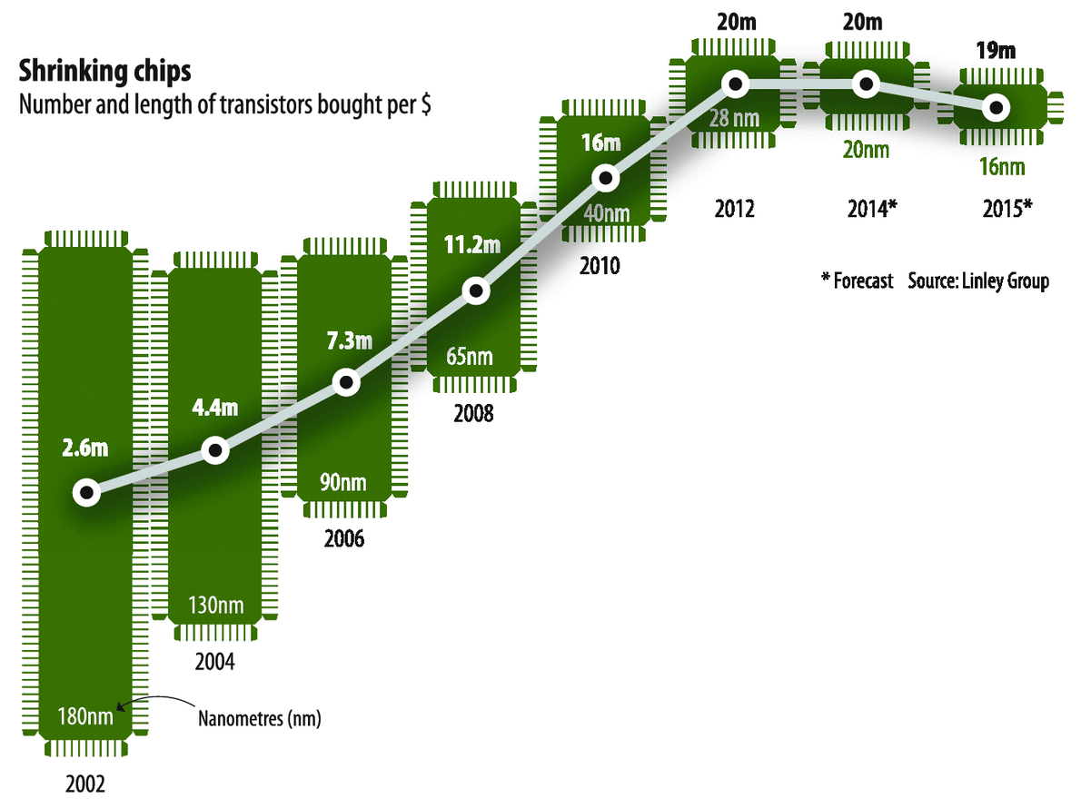
In the past, we could count on Moore's law (number of transistors in an integrated circuit to double every two years) to rely on major hardware improvements, resulting in substantially faster processors every few years.
However, recent microchip developments have stagnated.
Consequently, developing good code is more important now than ever before, as we can no longer rely on major hardware improvements.
This has led to a resurgence in both programming in fast compiled languages (such as C++) as well as parallel computing.
Moore's Law?

Why do I care?
My research consists of estimating high dimensional vector autoregressions
Consider a multivariate time series of dimensions \( T\times k \).
Let \( \{ \mathbf{y_t} \in \mathbb{R}^k\}_{t = 1}^T \) denote a \( k \) dimensional vector time series. A $p$th order vector autoregression (VAR\( _k \)(\( p \))) may be expressed as \[ \begin{align} &\mathbf{y}_t=\mathbf{\nu}+\sum_{\ell=1}^p\mathbf{B}_\ell\mathbf{y}_{t-\ell}+\mathbf{u}_t, \end{align} \]
- \( \mathbf{y}_t, \nu, \mathbf{u}_t \in \mathbb{R}^{k} \) for \( t=1,\dots,T \)
- each \( \mathbf{B}_{\ell} \) represents a \( k\times k \) coefficient matrix
- \( \mathbf{u}_t\stackrel{\text{wn}}{\sim}(\mathbf{0},\mathbf{\Sigma}_u) \)
- \( \mathbf{\Sigma}_u \) is nonsingular, but left unspecified in our analysis
In compact matrix representation, the aforementioned system is equivalent to \( \mathbf{Y}=\mathbf{\nu}\mathbf{1}^{'}+\mathbf{B}\mathbf{Z}+\mathbf{U} \) \[ \begin{align*} & \begin{array}[r]{lc} \mathbf{Y}=(\mathbf{y}_1,\mathbf{y}_2,\dots,\mathbf{y}_T),& (k\times T)\\ \mathbf{B}=(\mathbf{B}_1,\mathbf{B}_2,\dots,\mathbf{B}_p) & (k\times kp)\\ \mathbf{z}_t=(\mathbf{y}_{t-1}^{'},\dots \mathbf{y}_{t-p}^{'})^{'} & (kp\times 1)\\ \mathbf{Z}=(\mathbf{z}_1,\dots,\mathbf{z}_{T}) & (kp\times T)\\ \mathbf{U}=(\mathbf{u}_1,\dots,\mathbf{u}_T) & (k\times T)\\ \mathbf{1}=(1,\dots,1)^{'} & (T \times 1) \end{array} \end{align*} \]
The VAR takes the form \( \frac{1}{2}\|Y-BZ\|_F^2 \)
| Model Structure | Penalty | Solution Algorithm |
|---|---|---|
| Lasso | \( \lambda\|B\|_1 \) | Coordinate Descent |
| Lag Group Lasso | \( \lambda\sum_{\ell=1}^p||B_\ell||_F \) | Block Coordinate Descent |
| Own/Other Lag Group Lasso | \( \lambda(\rho_1\sum_{\ell=1}^p \|\text{diag}(B_{\ell})\|_F+\gamma_1\sum_{\ell=1}^p\|B_{\ell}^{-}\|_F) \) | Block Coordinate Descent |
| Lag Sparse Group Lasso | \( \lambda(1-\alpha) \sum_{\ell=1}^{p}\|B_{\ell}\|_{F}+\lambda\alpha\|B\|_{1} \) | Generalized Gradient Descent |
| Own/Other Sparse Group Lasso | \( \lambda(1-\alpha)[\rho_1\sum_{\ell=1}^p \|\text{diag}(B_{\ell})\|_F+\gamma_1\sum_{\ell=1}^p\|B_{\ell}^{-}\|_F]+\alpha\lambda\|B\|_{1} \) | Generalized Gradient Descent |
\( \lambda>0 \) is a penalty parameter estimated by cross-validation, \( 0\leq \alpha\leq 1 \) is an additional penalty parameter set to \( \frac{1}{k+1} \) to control within-group sparsity. \( \rho_1=\sqrt{k} \) and \( \gamma_1=\sqrt{k(k-1)} \) are weights accounting for the number of elements in each group.
Penalty Parameter selection
In order to account for time-dependence, cross-validation is conducted in a rolling manner. Define time indices \( T_1=\left \lfloor \frac{T}{3} \right\rfloor \), and \( T_2=\left\lfloor \frac{2T}{3} \right\rfloor \)
The training period \( T_1+1 \) through \( T_2 \) is used to select \( \lambda \),
\( T_2+1 \) through \( T \) is for evaluation of forecast accuracy in a rolling manner.

High-dimensional VARs
The coefficient matrix has dimension \( k\times kp \). If k=20 and p=12, that is 4800 parameters!
The Lasso doesn't have a closed form solution. The structured approaches don't even have closed form solutions for their one-block subproblems.
I have to re-estimate the entire coefficient matrix for a grid of \( \lambda \) values at every time point in the validation stage.
Hence, even in low dimensions, these problems can appear computationally intractible if coded inefficiently.
Memory
- Cache Hierarchy:
- Fast and expensive memory sits near the CPU
- As we get farther from the CPU, memory becomes larger, but slower
- The cache is located between the processor core and main memory.
- They contain copies of main memory blocks to speed up access to needed data.
- Respecting the underlying memory design can result in substantial performance improvements.
Locality
- Locality is an issue
- Spatial Locality: Things close together accessed consecutively
- Temporal Locality: Recently accessed data more likely to be accessed in the future.
- Latency and Bandwidth
- Latency: Time to finish a task
- Bandwidth: Number of tasks that can be completed in a fixed time
Different levels of memory
- L1 Cache: Located on the chip (one per core), very low latency (1cpu cycle 4-6 nanoseconds), high bandwidth (typically about 32kb or 4000 double precision numbers).
- L2 Cache: Larger (256kb, one per core), but higher latency (5-10 cycles)
- L3 Cache: Even Larger (6mb-shared by all cores), but higher latency (10-20 cycles). for more information.
- A contiguous block of data is stored in a cache line.
- If data requested by the processor is in a cache line, this is considered a “cache hit,” otherwise, it is a “cache miss.”
Why do we care?
- We probably aren't going to be doing low-level stuff like prefetching or writing sse instructions.
- However, we do work with matrices…
- R stores matrices in column-major order (i.e. consecutive elements of a column are stored in consecutive memory locations).
- If we subset an \( n\times n \) matrix by columns, this is cache coherent, as we are accessing consecutive elements in memory.
- Subsetting by rows is bad, as we are “walking” through the memory with a stride of n.
- Subsetting non-contiguous columns is bad, but not terrible, as each column is contiguous.
- Subsetting non-contiguous rows is the worst operation possible.
Example
library(microbenchmark)
A=matrix(runif(1e4^2),nrow=1e4,ncol=1e4)
test1=microbenchmark(
# Accessing 100 contiguous columns
B=A[,200:300],
## Accessing 100 contiguous rows, bad
B1=A[200:300,],
 #Accessing 99 non-contiguous rows, really bad
B2=A[seq(100,9900,by=100),],
 #Accessing 99 non-contiguous columns, doesn't matter that much..
B3=A[,seq(100,9900,by=100)],
  times=100L  )
Unit: milliseconds
 expr   min    lq  mean median    uq   max neval
    B 10.99 11.60 12.38  11.71 13.92 14.47   100
   B1 36.43 38.90 39.93  39.17 40.46 43.68   100
   B2 54.23 54.86 56.23  55.29 58.33 61.08   100
   B3 10.96 11.52 12.23  11.68 12.25 19.33   100

What do we do?
- If you are experiencing poor performance and can't figure out why, poor memory usage is a likely culprit.
- Perform operations by column, if possible.
- R is a dynamic language and it is very difficult to optimize memory usage (see Hadley's Chapter on Memory- basically avoid using data frames in loops).
- If you are working in a compiled language, consider the order of index variables in a loop.
- More advanced operations, such as blocking, compiler-level optimizations and sse instructions, can be considered if you get stuck.
- Monitor cache behavior with valgrind.
Moving on: Matrix Operations
- R and most modern programming languages rely on highly optimized matrix algorithms through an external FORTRAN library such as BLAS or LINPACK, which have been continuously refined since the 1970s.
- However, R's version of BLAS is a bit dated. Performance can be improved by linking to an external library such as OpenBLAS or Intel's Math Kernel Library, which have cache-optimized implementations and multithread support.
- Advantages: Doesn't require modification of existing code
- Disadvantages: Can be a pain to set up.
Efficient matrix operations
- The keys to efficient matrix operations are basically common sense
- Is your matrix positive definite? Use
chol2inv(chol(A))instead of solve(A) - Do you only need eigenvalues? Add the
only.valuesoption. - Avoid kronecker-type operations if possible.
- Learn a bit of matrix calculus
- Avoid doing unneccessary matrix operations in loops
- For some reason
crossprodandtcrossprodare almost always faster than %*%
- Is your matrix positive definite? Use
Sparse Matrices
One thing I haven't looked into are using sparse matrices.
They have advantages with respect to storage and matrix operations
The benefits are dependent upon the degree of sparsity.
Also, look-up costs become non-trivial!
Golub/Van Loan (or CS 6210) is a good source for learning efficient matrix algorithms.
Some Benchmarks
library(microbenchmark)
A=matrix(runif(1e2^2),nrow=1e2,ncol=1e2)
B=matrix(runif(1e2^2),nrow=1e2,ncol=1e2)
test1=microbenchmark(
B=t(A)%*%A,
B1=crossprod(A),
times=50L)
Unit: microseconds
 expr    min     lq   mean median     uq   max neval
    B 1284.7 1404.5 1876.3 1619.5 1966.5 12070    50
   B1  679.9  681.3  739.4  683.2  698.1  2926    50

A=matrix(runif(1e2^2),nrow=1e2,ncol=1e2)
A=t(A)%*%A
test1=microbenchmark(
B=solve(A),
B1=chol2inv(chol(A)),
B2=qr.solve(A),
times=50L
  )
Unit: microseconds
 expr    min     lq   mean median     uq  max neval
    B 2583.4 2622.9 2788.7 2650.7 2702.8 7821    50
   B1  747.5  769.7  976.7  781.8  801.3 9614    50
   B2 3584.8 3629.1 3764.6 3662.7 3785.7 5572    50

A=matrix(runif(1e2^2),nrow=1e2,ncol=1e2)
B=matrix(runif(1e2^2),nrow=1e2,ncol=1e2)
test1=microbenchmark(
C=A%*%B,
B1=crossprod(t(A),B),
times=50L
  )
Unit: milliseconds
 expr   min    lq  mean median    uq   max neval
    C 1.251 1.275 1.460  1.285 1.643 2.127    50
   B1 1.355 1.365 1.384  1.372 1.386 1.533    50

A=matrix(runif(1e2^2),nrow=1e2,ncol=1e2)
test1=microbenchmark(
C=eigen(A),
B1=eigen(A,only.values=TRUE),
times=50L
  )
Unit: milliseconds
 expr   min    lq  mean median    uq   max neval
    C 16.73 16.91 17.26  17.03 17.25 21.71    50
   B1 10.15 10.25 10.47  10.39 10.50 11.48    50

Profiling
- Once you get a working implementation of your code, it's a good idea to figure out where bottlenecks might be.
microbenchmarkcan be useful to compare different approaches, but R also has a good profiler than can give you some insight.
YYY <- MultVarSim(k,A,p,diag(k),nsims)
ZZZ <- Zmat2(YYY,p,k)
Z <- ZZZ$Z
Y <- ZZZ$Y
gran2=50
gamm <- LambdaGrid(40,gran2,Y,Z)
B <- betaCreate(k,p=2,gran2)
# microbenchmarking
Rprof()
op <- microbenchmark(
B1 <- lassoVAR(B,Z,Y,gamm,1e-3)
  ,times=50L)
Rprof(NULL)
summaryRprof()
$by.self
                self.time self.pct total.time total.pct
"lasso"              4.60    43.48       9.94     93.95
"%*%"                1.92    18.15       1.92     18.15
"ST"                 1.44    13.61       2.28     21.55
"seq"                0.52     4.91       0.90      8.51
"sum"                0.38     3.59       0.38      3.59
"seq.default"        0.22     2.08       0.34      3.21
"-"                  0.22     2.08       0.22      2.08
"FUN"                0.20     1.89       0.22      2.08
"*"                  0.18     1.70       0.18      1.70
"max"                0.18     1.70       0.18      1.70
"apply"              0.12     1.13       0.50      4.73
"mode"               0.12     1.13       0.12      1.13
"abs"                0.06     0.57       0.06      0.57
"gc"                 0.06     0.57       0.06      0.57
"sign"               0.06     0.57       0.06      0.57
"lassoVAR"           0.04     0.38      10.50     99.24
"unlist"             0.04     0.38       0.08      0.76
"match.fun"          0.04     0.38       0.04      0.38
".Call"              0.02     0.19      10.52     99.43
"lapply"             0.02     0.19       0.04      0.38
"any"                0.02     0.19       0.02      0.19
"aperm.default"      0.02     0.19       0.02      0.19
"matrix"             0.02     0.19       0.02      0.19
"mean.default"       0.02     0.19       0.02      0.19
"ncol"               0.02     0.19       0.02      0.19
"nrow"               0.02     0.19       0.02      0.19
"prod"               0.02     0.19       0.02      0.19

$by.total
                      total.time total.pct self.time self.pct
"block_exec"               10.58    100.00      0.00     0.00
"call_block"               10.58    100.00      0.00     0.00
"eval"                     10.58    100.00      0.00     0.00
"evaluate"                 10.58    100.00      0.00     0.00
"evaluate_call"            10.58    100.00      0.00     0.00
"handle"                   10.58    100.00      0.00     0.00
"in_dir"                   10.58    100.00      0.00     0.00
"knit"                     10.58    100.00      0.00     0.00
"microbenchmark"           10.58    100.00      0.00     0.00
"process_file"             10.58    100.00      0.00     0.00
"process_group"            10.58    100.00      0.00     0.00
"process_group.block"      10.58    100.00      0.00     0.00
"withCallingHandlers"      10.58    100.00      0.00     0.00
"withVisible"              10.58    100.00      0.00     0.00
".Call"                    10.52     99.43      0.02     0.19
"lassoVAR"                 10.50     99.24      0.04     0.38
"lasso"                     9.94     93.95      4.60    43.48
"ST"                        2.28     21.55      1.44    13.61
"%*%"                       1.92     18.15      1.92    18.15
"seq"                       0.90      8.51      0.52     4.91
"apply"                     0.50      4.73      0.12     1.13
"sum"                       0.38      3.59      0.38     3.59
"seq.default"               0.34      3.21      0.22     2.08
"-"                         0.22      2.08      0.22     2.08
"FUN"                       0.22      2.08      0.20     1.89
"*"                         0.18      1.70      0.18     1.70
"max"                       0.18      1.70      0.18     1.70
"mode"                      0.12      1.13      0.12     1.13
"unlist"                    0.08      0.76      0.04     0.38
"abs"                       0.06      0.57      0.06     0.57
"gc"                        0.06      0.57      0.06     0.57
"sign"                      0.06      0.57      0.06     0.57
"match.fun"                 0.04      0.38      0.04     0.38
"lapply"                    0.04      0.38      0.02     0.19
"any"                       0.02      0.19      0.02     0.19
"aperm.default"             0.02      0.19      0.02     0.19
"matrix"                    0.02      0.19      0.02     0.19
"mean.default"              0.02      0.19      0.02     0.19
"ncol"                      0.02      0.19      0.02     0.19
"nrow"                      0.02      0.19      0.02     0.19
"prod"                      0.02      0.19      0.02     0.19
"aperm"                     0.02      0.19      0.00     0.00

$sample.interval
[1] 0.02

$sampling.time
[1] 10.58
Profiling
Profiling gives you an idea of where your program spends the most amount of time
This can give you some insight as to either how to optimize your code within R or move it to C++.
For example, this procedure spends a lot of time in the Soft-Threshold function. This can easily be ported to C++.
Alternatively, I could use vectorized operations… What will be faster?
Unit: milliseconds
                                     expr    min     lq   mean median
   Orig <- lassoVAR(B, Z, Y, gamm, 0.001) 102.29 103.38 106.52 104.35
   Cpp <- lassoVAR2(B, Z, Y, gamm, 0.001) 103.83 105.68 109.01 106.50
 Vec <- lassoVARVec(B, Z, Y, gamm, 0.001)  47.67  49.29  51.59  52.27
     uq    max neval
 107.54 164.74    50
 109.74 164.07    50
  52.85  55.75    50

Vectorizing
- It's clear that vectorizing code helps a lot, but I still don't like doing it.
- Why? The code becomes difficult to read/interpret and its an unnatural coding practice.
- Moreover, if you port your code to a compiled language, you'll just have to rewrite it in its previous form!
Let's see what the performance difference is between vectorized code and C++ code
Unit: milliseconds
                                         expr    min     lq   mean median
       Orig <- lassoVAR(B, Z, Y, gamm, 0.001) 391.20 394.92 399.00 396.76
     CppST <- lassoVAR2(B, Z, Y, gamm, 0.001) 396.54 402.92 407.76 405.53
     Vec <- lassoVARVec(B, Z, Y, gamm, 0.001) 162.85 165.80 166.91 166.83
 FullCpp <- lassoVARCPP(B, Z, Y, gamm, 0.001)  33.81  34.66  35.83  35.22
     uq    max neval
 398.81 449.27    50
 408.60 460.06    50
 167.64 173.49    50
  36.48  40.47    50

Algorithms
There are many algorithms that can be used as solution methods for the Lasso
- Coordinate Descent, Generalized Gradient Descent, Gauss-Seidel, calls to convex optimization solvers, etc
Which one is going to be the fastest? Generally, it is context dependent.
Unit: milliseconds
                                                     expr    min     lq
                  CD <- lassoVARCPP(B, Z, Y, gamm, 0.001) 19.639 19.778
 FISTA <- .lassoVARFist(B1a, Z, Y, gamm, 0.001, p, FALSE)  4.815  4.856
   mean median     uq    max neval
 20.314 20.129 20.670 21.887    25
  4.932  4.923  4.976  5.161    25

Rcpp
Provides an interface to C++ which lets you directly incorporate R data structures.
Can be done inline or via
sourceCppDoesn't require that much knowledge of C++ to use effectively
Also provides an interface to the
Armadillonumerical linear algebra library, which allows for fast and relatively painless matrix operations.I started using Rcpp in August 2013 with no knowledge of C++
- My R package now has over 2000 lines of C++ which allows for my methods to actually run in high dimensions.
Rcpp
The general strategy to port to C++ is to start from the inside and work your way out.
What results in the biggest performance gains?
- Explicit for loops, basically any iterative process
- Most things recognized by the profiler as bottlenecks
- Exclusively matrix operations will probably not make much of a difference.
Can you profile Rcpp code? Yes, but it requires a bit of work.
Avoiding Bottlenecks using Rcpp
The interface between R and C++ has some overhead. Avoid calling a C++ function multiple times from R.
PASS BY REFERENCE!!! This is one the biggest time-sinks in R. All functions pass by value. You can avoid this in Rcpp by adding
&before Armadillo object and_after an Rcpp object.Don't try to be fancy. Take advantage of of Rcpp and Armadillo's functionality (remember rule 2).
Parallel Computing
Since microchip development has been relatively stagnant, attention has instead been shifted to distributed computing, as most modern computers have multiple cores.
By linking external BLAS libraries, R has some multithreaded support, but it is primarily single threaded.
If you convert all of your Rcpp objects to Armadillo or Native C++ objects, you can utilize OpenMP within C++ to parallelize for loops.
There is also a package
RcppParallelin development.
Parallel Computing in R
Within R, there are facilities for parallel computing in packages
snow,foreach,doMC,etc.These procedures involving spawning separate R processes and aggregating the data.
Aggregated data are usually stored in lists that will need to be collapsed.
Implementation
On your own system, parallel code might look something like this
- See Parallelex.R script
Parallel Computing on a cluster
We have a computing cluster available for research
It has 30 nodes each with 8 processors
Slightly different than parallel computing on your own machine
More care is required when setting up the cluster, as you will need the addresses of nodes.
Typically, you write a bash script and run it through a scheduler rather than run R code directly.
Unfortunately, the cluster is fairly dated and technical issues need to be addressed with CAC.
Amazon Ec2
As an alternative, it is possible to create an “on-demand” cluster using Amazon Ec2.
One can create virtual “instances,” each of which can be thought of as one “node” of a cluster
You have full control over these instances and can create up to 20 at a time.
You don't need to use a scheduler, you will instead execute your script with something like
nohup R CMD BATCH Script.R Res.txt &
Conclusion/Reflections
Though R has severe limitations, through good coding practices it is possible to achieve good performance.
We will not be using R forever. Hopefully the eventual successor will correct its flaws.
Julia looks particularly promising, but in my opinion, it is still too experimental for everyday use.
References
- Hadley Wickham's Advanced R
- Stack Overflow, Mailing lists (e.g. rcpp-devel), etc
- My Blog