Data Analysis and Visualization - Lesson 2
alper yilmaz
September 26th, 2017
Hi again. I hope you enjoyed the “Introduction to R” course throughout last week. Now, you have fair understanding of R programming language.
Review of last week
Let’s do some exercises for refreshing our memories.
##

# Please fix the code
instructor name <- alper yilmaz

##

# What is the data type of the variable x_3?

> str(df1)
'data.frame':   5 obs. of  5 variables:
 $ x_1: int  14 33 36 43 12
 $ x_2: num  41 29 10 5 27
 $ x_3: chr  "R" "P" "J" "N" ...
 $ x_4: Factor w/ 5 levels "April","December",..: 3 5 4 1 2
 $ x_5: logi  FALSE FALSE TRUE TRUE FALSE

##

# Complete the script to produce the output shown

#OUTPUT
[1] "C" "D"

#SCRIPT
store <- list(prod = c("C", "D"), cost = c(15, 20))
store_________ (use brackets only)

##

# Complete the script to produce the output shown

# OUTPUT
[1] 2

# SCRIPT
x <- c(1, 2, 3)
# Find the average of x

_______(x)
DataCamp also provides daily exercises if you are interested in daily short exercises (slow but steady wins the race). Here’s the link for “Introduction to R” daily exercise. Let’s head over and do a small exercise.
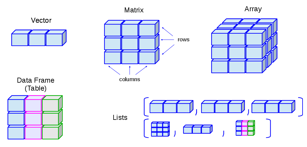
R data structures
The image below concisely illustrates the different type of data structures in R.

R data structures
(Source: http://venus.ifca.unican.es/Rintro/_images/dataStructuresNew.png)
Running code in RStudio
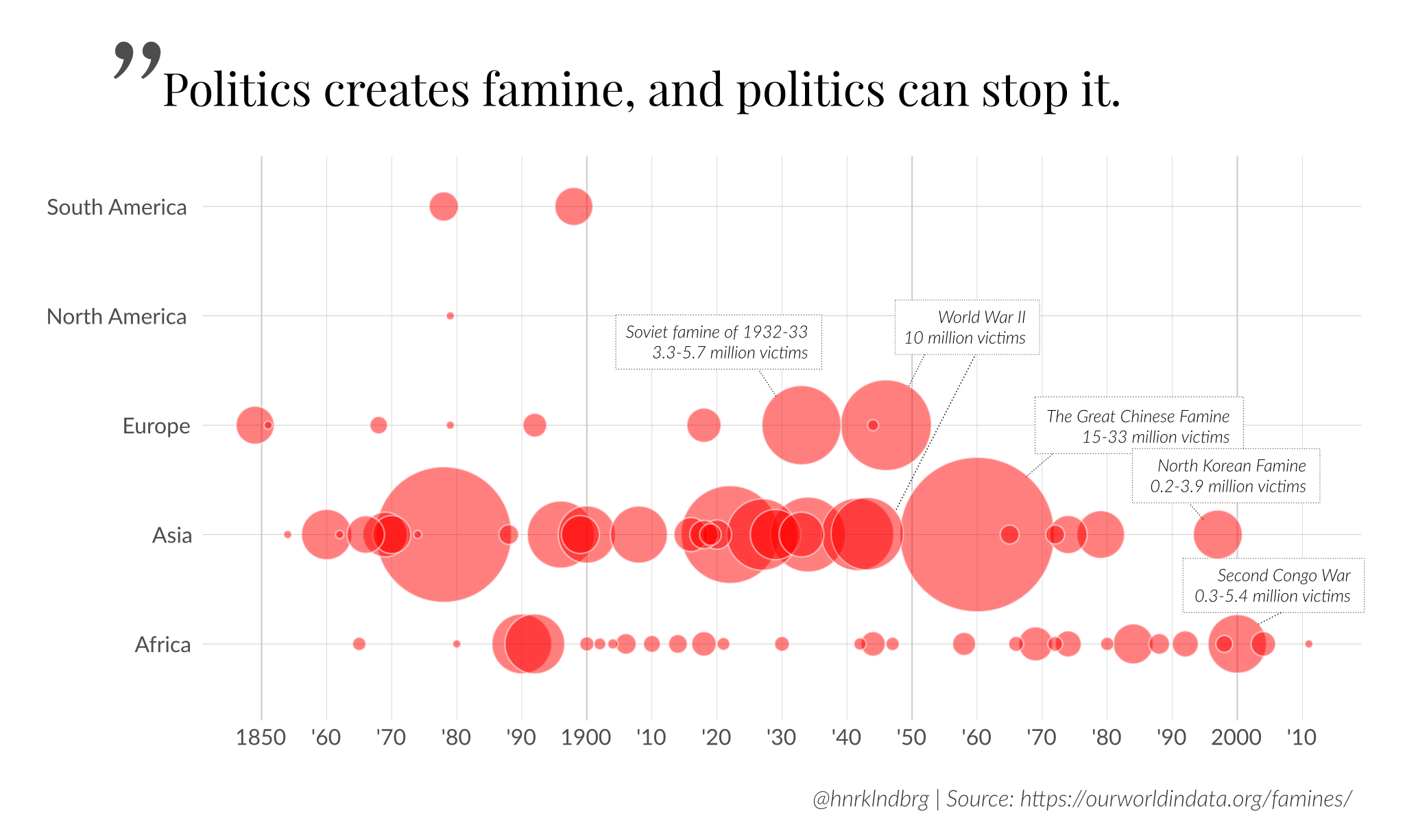
Let’s copy paste the code below to your Rstudio and run it (link actual code source). The result should be as shown below the code. The code is taken from Github repo of Henrik Lindberg, en expert in data visualization.
But wait, where do you paste this code? Running it line by line in console won’t feasible. Let’s open a new R script file and paste the code there.
As you remember from last week and DataCamp environment, we can use some keyboard shortcuts to run code in code panel. Ctrl+Enter can be used to run the code in the line where cursor is located. Ctrl+Shift+Enter runs the whole code if you are insterested running the code at once. Also, if you want to run multiple (consecutive) lines, you can select them and press Ctrl+Enter keys.
library(tidyverse)
library(rvest)

SOURCE='https://ourworldindata.org/famines/'

h <- read_html(SOURCE)
h %>%
  html_table() %>%
  .[[1]] %>%
  mutate(year_start = as.integer(substring(Year, 1, 4)),
         year_end = as.integer(substring(Year, 6)),
         digits = ceiling(log10(year_end)),
         year_end = as.integer(floor(year_start / 10^digits) * 10^digits + year_end),
         year_end = coalesce(year_end, year_start)) %>%
  select(-digits) %>%
  mutate(mortality = as.numeric(gsub(',', '', `Excess Mortality- mid-point`))) %>%
  transmute(year_start, year_end, mortality, country=Country, continent=`OWID continent`) %>%
  mutate(continent = recode(continent, 'Europe/Asia' = 'Asia')) %>%
  group_by(continent, year = round((year_start + year_end)/2)) %>%
  summarize(mortality = sum(mortality, na.rm=TRUE)) %>%
  filter(continent != '') %>%
  arrange(-mortality) %>%
  ggplot(aes(year, continent, size=mortality)) +
  geom_point(alpha=0.5, fill='red', color='white', shape=21) +
  scale_size_continuous(range=c(1, 25), breaks=c(1, 10, 20)*1e6) +
  scale_x_continuous(breaks=seq(from=1850, to=2015, by=10), labels=function(x) {ifelse(x %% 100 == 0 | x == 1850, paste0(x), paste0("'", x%%100))}) +
  labs(x="", y="", title="Famines", caption=paste0("@hnrklndbrg | Source: ", SOURCE))
## Warning in evalq(as.integer(substring(Year, 6)), <environment>): NAs
## introduced by coercion
This image is (nearly) identical to what was drawn by the original author (see below)

Original famine image
This is reproducible research in action! Please refer to “About reproducible research” section.
Running and editing multiple files
In RStudio, you can visit a folder full of script files (or an Rproject folder) and in that case you can view contents of them or run them.
Let’s clone viz-pub repo from Github into our Rstuido session. Please refer to “About Git and Github” section for details. The git repository url is https://github.com/halhen/viz-pub.git
File --> New Project --> Version Control --> Git --> Paste URL (you can choose new session)In Files tab of right bottom pane, you can see that all folders and contents within them are copied. code.R or .Rmd files in following folders can be run directly or with slight modifications (working directory issue)

Setting working directory
“Working directory” concept is quite important when reading or writing files. In such operations RStudio has to know from which folder to read. You can check the current working directory with getwd() command. In the example above, code.R file imports csv files and thus RStudio needs know to check the current folder contents while importing files.
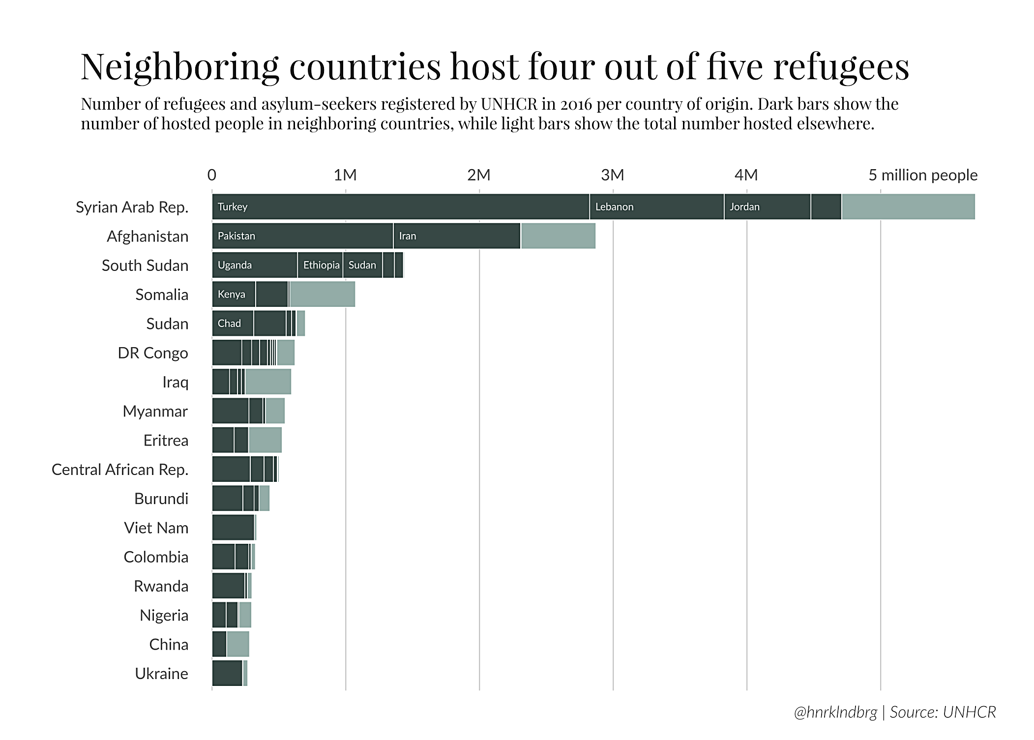
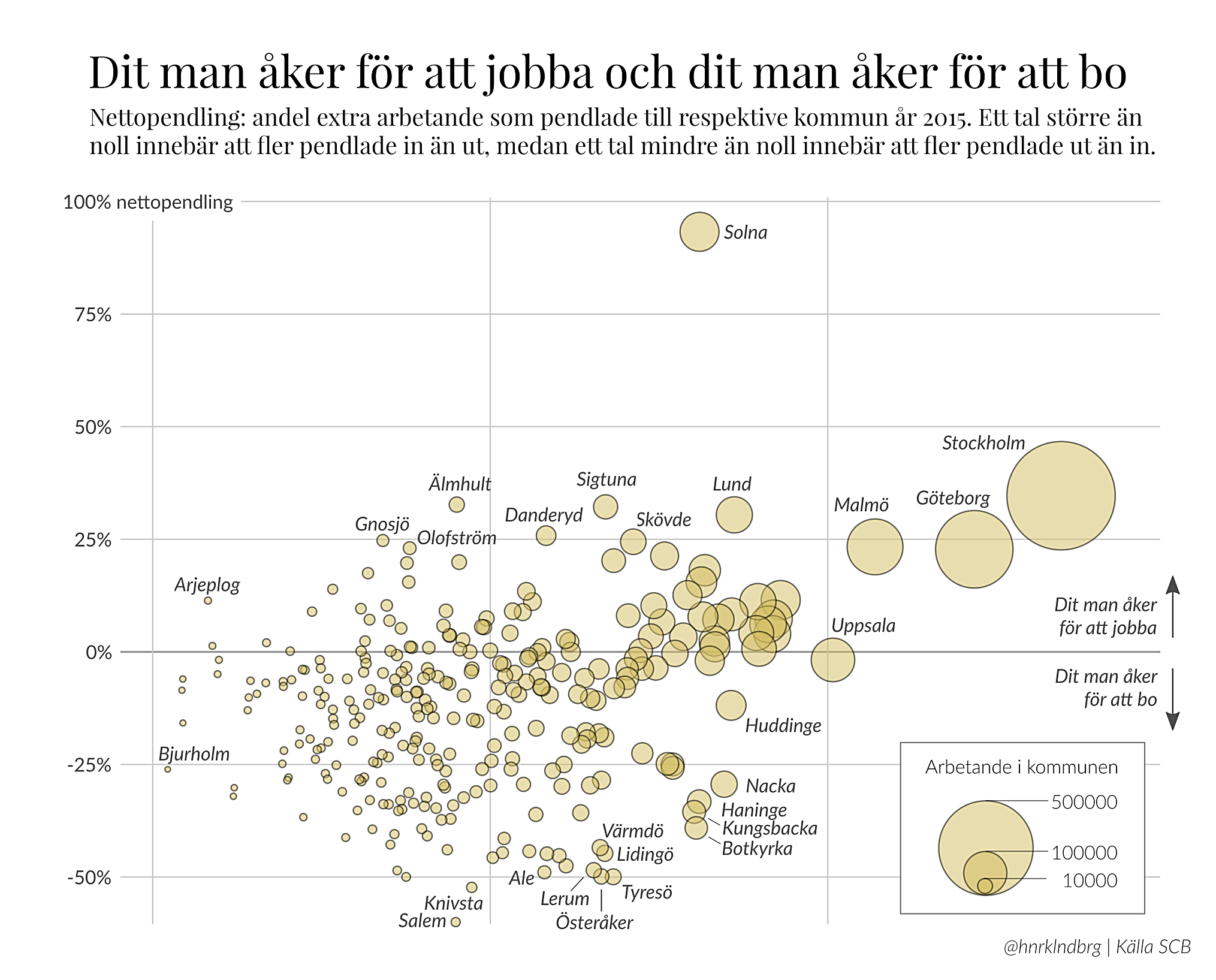
Let’s try to visit and run following folder contents:
- famine (already run above) (folder - image)
- refugee-neighbor (folder - image)
- se-commuting (folder - image)
- some-countries (Rmd file - pyramids only) (folder - image)
- sports-depeche (Rmd file - think outside the box) (folder - image)
- water (folder - image)
Please visit other folders and check out the outputs. As you can see, ggplot2 is quite capable visualization tool.
Please note that the author produces SVG formatted file and version controls the changes in SVG as well. SVG file, although it’s scalable vector graphics, is actually a plain text format.
Please go over the svg code below and the image it generates.
<svg xmlns:svg="http://www.w3.org/2000/svg"
xmlns:xlink="http://www.w3.org/1999/xlink"
version="1.1" width="500" height="200">

<circle cx="164" cy="62.1" r="53.8"
style="fill:#ff6600;stroke-width:9.5;stroke:#902100"/>

<text xml:space="preserve" style="fill:#808080;font-family:Arial;
font-size:62.5px;letter-spacing:12.09;line-height:125%;
text-align:start;text-anchor:start;word-spacing:0px">
  <textPath xlink:href="#path4241">Sample Text</textPath>
</text>

<path d="M 286.51,96.29 401.02,29.34"
style="fill:none;stroke-width:3.20;stroke:#57bf85"/>

<text xml:space="preserve" x="270.46" y="109.56"
style="font-family:Arial;font-size:25px">a</text>

<text xml:space="preserve" x="404.35" y="29.49"
style="font-family:Arial;font-size:25px">b</text>

<path
     id="path4241"
     d="m 37.014436,107.42857 c 0,0 226.190484,199.73545 425.925934,0"
     style="fill:none;fill-rule:evenodd;stroke:#00a0df;stroke-width:2;
     stroke-opacity:0.94117647" />
</svg>
The SVG code above produces the image below:

SVG image sample
Normally, SVG files can be viewed by many image viewers, but if you’re interested in editing them you need vector graphics softwares such as Inkscape or Adobe Illustrator. If you want to quickly render and play with svg file, you can try at svg-editor online. Please visit SVG Pocket Guide in order to get more insight about how SVG is rendered.
Below is the magnification of png version:

PNG zoom
And below is the zoom in versions of same image in SVG (matching region and even more zooming)

SVG zoom into same region

Even more zoom into same region in SVG
About reproducible research
The quote below is taken from Motivation section at http://reproducibleresearch.net/.
After a colleague asked something about a paper you wrote, you spend a considerable amount of time finding back the right program files you used in that paper. Not to talk about the time to get back to the set of parameters used to produce that nice result.
There are quite number of research articles listed here.
The book titled “Reproducible Research with R and R Studio, Second Edition” discussed how reproducible research can be achieved with R.
The ReScience Journal is a peer-reviewed journal that targets computational research and encourages the explicit replication of already published research, promoting new and open-source implementations in order to ensure that the original research is reproducible.

ReScience Journal logo
About Git and Github
Git is an open-source version control system and Github is where developers store their projects and network with like minded people. In Github, plain text content (code, report, article, etc.) is kept and version controlled by Git.
Github can be used as publishing platform, which means goodbye to “final_final_v2.doc” or “en_enson_final_09252017.doc”

phdcomics final.doc
Github serves not only code but also interacts with it with integration tools. It can test your code, trigger actions after code changes and it can deploy after testing. Also, Github can serve static html pages and thus can be used as blogging platform. We’ll be using blogdown to publish our analysis and code. Here’s a website served on Github and here’s the code for the same website.
In Github, for a repo, it’s possible to:
Assignments for next week
In the first code example, we notice essential components of data analysis and visualization. Importing data (from URL, file, etc.), manupulating data and finally visualizing data. Let’s learn basics about each component.
Assignments until next Monday:
- Importing Data Into R (Part 1) - Chapter 1 - Importing data from flat files with utils
- Data Manipulation in R with dplyr - Chapter 1 - Introduction to dplyr and tbls
- Data Visualization with ggplot2 (Part 1) - Chapter 1 - Introduction