DATA606 Linear Regression Presentation
Kyle Gilde
4/20/2017
Linear Regression & Murder!

7.29 Murders and Poverty, Part I.
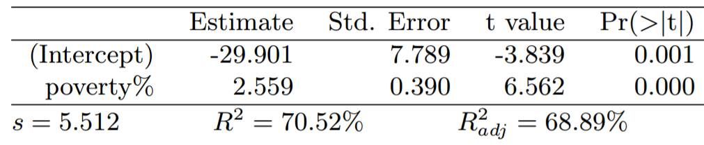
The following regression output is for predicting annual murders per million from the percentage living in poverty in a random sample of 20 metropolitan areas.
5-Part Question
(a) Write out the linear model.
A linear model is expressed as \( y = {\beta}_{1}x + {\beta}_{0} \) where \( {\beta}_{1} \) is the slope of the line and \( {\beta}_{0} \) is the line's y-intercept.
From the Estimate column of the regression output, we know that \( {\beta}_{0} = -29.901 \) and is the line's y-intercept. \( {\beta}_{1} = 2.559 \) and is the slope of the line.
Consequently, the linear model for the murder rate as a function of the poverty rate is expressed as \( \widehat{murder} = -29.901 + 2.559*{poverty\%} \)
Conditions for Least Squares Line
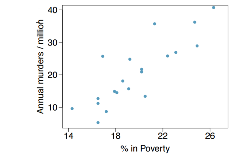
Before continuing, let's stop & check to the best of our ability given that we only have the scatter plot and not the raw data that the conditions for least-squares regression have been met.
Check of Conditions
- Linearity: The points in the plot do show a linear trend.
- Nearly normal residuals: From the scatter plot, we don't see any outlying points.
- Homoscedasticity (aka constant variability): Having only the scatter plot, the points appear to have constant variability.
- Independent observations: The data are from a random sample, and they are not from a time series.