- Introduce R by example
- Highlight useful data manipulation functions
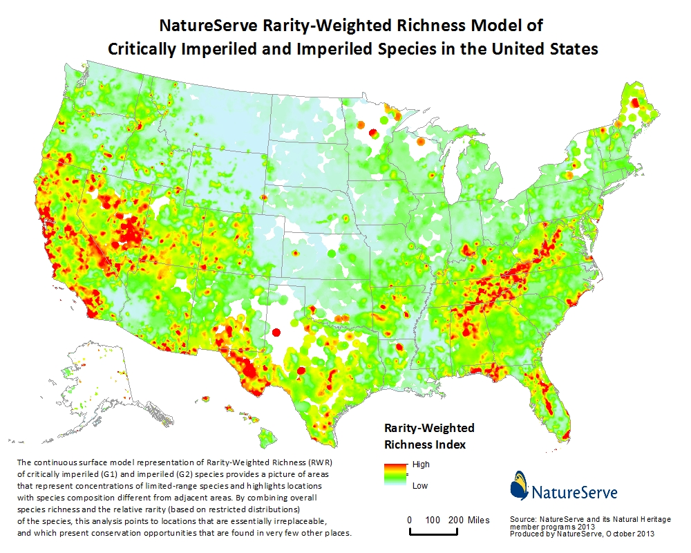
- Demonstrate methods for working with spatial data
- Increase familiarity with climate data
March 16, 2017
Goals:
Federally listed species in California: https://ecos.fws.gov/ecp0/reports/species-listed-by-state-report?state=CA&status=listed
Getting started
Set working directory:
setwd("/Volumes/collnell/CAT/") ##change location to your folder
getwd() #tells you what the current directory is
## [1] "/Volumes/collnell/CAT"
Windows: make sure to use '/'
Read in data
Download data files:
https://drive.google.com/drive/folders/0B-TN-iTwt6b3eHRMREpyZU8yWXM?usp=sharing
listed_sp_ca
end_sp_df
Read in data
list_url<-'https://drive.google.com/file/d/0B-TN-iTwt6b3X3E2VzhUanQyOU0/view?usp=sharing'
end_url<-'https://drive.google.com/file/d/0B-TN-iTwt6b3T1k2cjg2dnlQMFU/view?usp=sharing'
##for the following to work, need to make the folders to download in
##OR go to the url and manually download the file, and change the path after 'read.csv'
download.file(list_url, destfile='data/ENV/listed_sp_ca.csv')
download.file(end_url, destfile='data/ENV/end_sp_ca.csv')

listed<-read.csv('data/ENV/listed_sp_ca.csv')
str(listed) ##structure of the data
## 'data.frame':    275 obs. of  8 variables:
##  $ Status              : Factor w/ 2 levels "E","T": 1 1 2 1 2 1 1 1 1 1 ...
##  $ Species.Listing.Name: Factor w/ 275 levels "Abalone, White\xe5\xcaNorth America (West Coast from Point Conception, CA, U.S.A., to Punta Abreojos, Baja California, Mexico) "| __truncated__,..: 1 2 15 12 13 14 32 39 31 40 ...
##  $ kingdom             : Factor w/ 2 levels "animal","plant": 1 1 1 1 1 1 1 1 1 1 ...
##  $ organism            : Factor w/ 157 levels "Abalone","Albatross",..: 1 2 10 10 10 10 19 19 19 19 ...
##  $ species             : Factor w/ 269 levels "Acanthomintha ilicifolia",..: 147 204 94 95 112 215 14 48 127 128 ...
##  $ rank                : Factor w/ 2 levels "SPECIES","SUBSPECIES": 1 1 2 1 1 1 2 2 2 2 ...
##  $ class               : Factor w/ 12 levels "Actinopterygii",..: 5 3 6 6 6 6 6 6 6 6 ...
##  $ taxonkey            : int  2293070 2481385 4292518 1054051 1035540 1057467 1934362 4300277 4300212 1926009 ...
class(listed$Status)
## [1] "factor"
levels(listed$Status) ##show levels of a factor
## [1] "E" "T"
dplyr: A grammar of data manipulation
install.packages('dplyr')
library(dplyr)
Verbs
+ filter() - subset rows
+ select() - subset columns
+ join() - combine dataframe
+ group_by() & summarize() - summarize rows
+ mutate() - make new columns
+ arrange() - reorder rows
filter()
Subset rows of a dataframe
dim(listed)
## [1] 275 8
end_animals<-filter(listed, Status == 'E', kingdom != 'plant')
#'!' in front means 'is not equal to'
dim(end_animals)
## [1] 81 8
Returns endangered species (E) only.
select()
Select columns of a dataframe:
df<-select(end_animals, kingdom, organism, species, rank, class) #select columns
head(df)
##   kingdom  organism                    species       rank      class
## 1  animal   Abalone         Haliotis sorenseni    SPECIES Gastropoda
## 2  animal Albatross       Phoebastria albatrus    SPECIES       Aves
## 3  animal    Beetle            Dinacoma caseyi    SPECIES    Insecta
## 4  animal    Beetle         Polyphylla barbata    SPECIES    Insecta
## 5  animal Butterfly      Apodemia mormo langei SUBSPECIES    Insecta
## 6  animal Butterfly Callophrys mossii bayensis SUBSPECIES    Insecta
df<-select(end_animals, -Species.Listing.Name, -taxonkey) #Deselect columns
colnames(df)
## [1] "Status" "kingdom" "organism" "species" "rank" "class"
Error: unable to find an inherited method for function 'select'
Try 'dplyr::select()'
Pipes
%>%
- Connects series of code on the same object
- 'and then'
df<-listed %>% #original df
  filter(Status == 'E', kingdom != 'plant') %>%
  select(kingdom:class)  #columns kingdom through class

head(df)
##   kingdom  organism                    species       rank      class
## 1  animal   Abalone         Haliotis sorenseni    SPECIES Gastropoda
## 2  animal Albatross       Phoebastria albatrus    SPECIES       Aves
## 3  animal    Beetle            Dinacoma caseyi    SPECIES    Insecta
## 4  animal    Beetle         Polyphylla barbata    SPECIES    Insecta
## 5  animal Butterfly      Apodemia mormo langei SUBSPECIES    Insecta
## 6  animal Butterfly Callophrys mossii bayensis SUBSPECIES    Insecta
Joins

Combine multiple dataframes based on common values.
Joins
#Read in new data
sp.occ<-read.table('data/ENV/end_sp_df.csv', header = TRUE, sep = ",")

sp.occ$Long<-sp.occ$decimalLongitude
sp.occ$Lat<-sp.occ$decimalLatitude
sp.occ<-sp.occ%>%select(-decimalLongitude, -decimalLatitude)

str(sp.occ)#species observations in CA from 2007-2017
## 'data.frame':    82104 obs. of  8 variables:
##  $ name         : Factor w/ 195 levels "Acanthomintha ilicifolia",..: 150 150 150 150 150 150 150 150 150 150 ...
##  $ basisOfRecord: Factor w/ 5 levels "HUMAN_OBSERVATION",..: 1 1 1 1 1 1 1 1 1 1 ...
##  $ year         : int  2015 2014 2014 2014 2014 2014 2014 2014 2014 2014 ...
##  $ month        : int  8 2 2 2 2 2 2 2 2 2 ...
##  $ day          : int  15 22 22 22 22 22 22 22 22 22 ...
##  $ taxonkey     : int  2481385 2481385 2481385 2481385 2481385 2481385 2481385 2481385 2481385 2481385 ...
##  $ Long         : num  -125 -125 -125 -125 -125 ...
##  $ Lat          : num  48.4 44.5 44.5 44.5 44.5 ...
Joins
#join by variables with different names
sp.df<-left_join(sp.occ, listed, by=c('name'='species'))
##join species from listed that occur in sp.occ
sp.df<-left_join(sp.occ, listed, by='taxonkey')
colnames(sp.df)
##  [1] "name"                 "basisOfRecord"        "year"
##  [4] "month"                "day"                  "taxonkey"
##  [7] "Long"                 "Lat"                  "Status"
## [10] "Species.Listing.Name" "kingdom"              "organism"
## [13] "species"              "rank"                 "class"
group_by() & summarize()
How many observations are there for each class?
sp.class<-sp.df%>%
  filter(Status == 'E')%>%
  dplyr::group_by(kingdom, class)%>%
  summarize(obs_n= length(species)) #count of obs

sp.class
## Source: local data frame [10 x 3]
## Groups: kingdom [?]
##
##    kingdom          class obs_n
##     <fctr>         <fctr> <int>
## 1   animal Actinopterygii 16627
## 2   animal       Amphibia   787
## 3   animal           Aves 22706
## 4   animal   Branchiopoda    33
## 5   animal        Insecta   981
## 6   animal   Malacostraca     4
## 7   animal       Mammalia  2405
## 8   animal       Reptilia   355
## 9    plant     Liliopsida   185
## 10   plant  Magnoliopsida  2413
mutate & arrange()
Which class has the most observtions? Approximately how many observations are there per species within each class?
sp.class<-sp.df%>%
  filter(Status == 'E')%>%
  dplyr::group_by(kingdom, class)%>%
  summarize(sps_n = length(unique(taxonkey)),
            obs_n= length(species))%>%
  arrange(desc(obs_n))%>% #sort in descnding order
  mutate(obs_sp = obs_n/sps_n)
head(sp.class)
## Source: local data frame [6 x 5]
## Groups: kingdom [2]
##
##   kingdom          class sps_n obs_n     obs_sp
##    <fctr>         <fctr> <int> <int>      <dbl>
## 1  animal           Aves     7 22706 3243.71429
## 2  animal Actinopterygii     8 16627 2078.37500
## 3   plant  Magnoliopsida    75  2413   32.17333
## 4  animal       Mammalia    17  2405  141.47059
## 5  animal        Insecta    12   981   81.75000
## 6  animal       Amphibia     5   787  157.40000

Challenge
How many federally listed species have no records in the last 20 years? Which ones?
gone<-sp.occ%>%
  full_join(listed, by=c('name'='species'))%>% #full keeps rows from listed w/ no obs
  filter(is.na(year))%>%
  group_by(name)

length(gone$name)
## [1] 157
gone$name
##   [1] "Haliotis sorenseni"
##   [2] "Desmocerus californicus dimorphus"
##   [3] "Dinacoma caseyi"
##   [4] "Apodemia mormo langei"
##   [5] "Callophrys mossii bayensis"
##   [6] "Euphilotes battoides allyni"
##   [7] "Euphilotes enoptes smithi"
##   [8] "Euphydryas editha bayensis"
##   [9] "Euphydryas editha quino"
##  [10] "Glaucopsyche lygdamus palosverdesensis"
##  [11] "Icaricia icarioides missionensis"
##  [12] "Lycaeides argyrognomon lotis"
##  [13] "Speyeria callippe callippe"
##  [14] "Speyeria zerene behrensii"
##  [15] "Speyeria zerene hippolyta"
##  [16] "Speyeria zerene myrtleae"
##  [17] "Gila bicolor snyderi"
##  [18] "Gila elegans"
##  [19] "Pacifastacus fortis"
##  [20] "Streptocephalus woottoni"
##  [21] "Rhaphiomidas terminatus abdominalis"
##  [22] "Empidonax traillii extimus"
##  [23] "Urocyon littoralis catalinae"
##  [24] "Vulpes macrotis mutica"
##  [25] "Polioptila californica californica"
##  [26] "Trimerotropis infantilis"
##  [27] "Dipodomys heermanni morroensis"
##  [28] "Dipodomys merriami parvus"
##  [29] "Dipodomys nitratoides exilis"
##  [30] "Dipodomys nitratoides nitratoides"
##  [31] "Dipodomys stephensi"
##  [32] "Gambelia silus"
##  [33] "Lynx canadensis"
##  [34] "Aplodontia rufa nigra"
##  [35] "Perognathus longimembris pacificus"
##  [36] "Enhydra lutris nereis"
##  [37] "Strix occidentalis caurina"
##  [38] "Ptychocheilus lucius"
##  [39] "Charadrius alexandrinus nivosus"
##  [40] "Cyprinodon radiosus"
##  [41] "Sylvilagus bachmani riparius"
##  [42] "Rallus longirostris levipes"
##  [43] "Rallus longirostris obsoletus"
##  [44] "Rallus longirostris yumanensis"
##  [45] "Ambystoma macrodactylum croceum"
##  [46] "Batrachoseps aridus"
##  [47] "Lepidochelys olivacea"
##  [48] "Ovis canadensis nelsoni"
##  [49] "Ovis canadensis sierrae"
##  [50] "Sorex ornatus relictus"
##  [51] "Lanius ludovicianus mearnsi"
##  [52] "Pseudocopaeodes eunus obscurus"
##  [53] "Pyrgus ruralis lagunae"
##  [54] "Hypomesus transpacificus"
##  [55] "Helminthoglypta walkeriana"
##  [56] "Thamnophis sirtalis tetrataenia"
##  [57] "Amphispiza belli clementeae"
##  [58] "Gasterosteus aculeatus williamsoni"
##  [59] "Acipenser medirostris"
##  [60] "Catostomus santaanae"
##  [61] "Xyrauchen texanus"
##  [62] "Sterna antillarum browni"
##  [63] "Pipilo crissalis eremophilus"
##  [64] "Oncorhynchus aguabonita whitei"
##  [65] "Oncorhynchus clarkii henshawi"
##  [66] "Oncorhynchus clarkii seleniris"
##  [67] "Gila bicolor  mohavensis"
##  [68] "Vireo bellii pusillus"
##  [69] "Microtus californicus scirpensis"
##  [70] "Balaenoptera borealis"
##  [71] "Physeter catodon"
##  [72] "Neotoma fuscipes riparia"
##  [73] "Plagiobothrys strictus"
##  [74] "Alopecurus aequalis  sonomensis"
##  [75] "Berberis pinnata  insularis"
##  [76] "Galium buxifolium"
##  [77] "Galium californicum  sierrae"
##  [78] "Cordylanthus palmatus"
##  [79] "Cordylanthus maritimus  maritimus"
##  [80] "Cordylanthus mollis  mollis"
##  [81] "Cordylanthus tenuis  capillaris"
##  [82] "Lesquerella kingii  bernardina"
##  [83] "Trichostema austromontanum  compactum"
##  [84] "Poa napensis"
##  [85] "Brodiaea pallida"
##  [86] "Eriogonum apricum"
##  [87] "Senecio layneae"
##  [88] "Eryngium aristulatum  parishii"
##  [89] "Opuntia treleasei"
##  [90] "Ceanothus ferrisae"
##  [91] "Sidalcea oregana  valida"
##  [92] "Clarkia imbricata"
##  [93] "Clarkia speciosa  immaculata"
##  [94] "Trifolium amoenum"
##  [95] "Cupressus abramsiana"
##  [96] "Dudleya abramsii  parva"
##  [97] "Dudleya cymosa  marcescens"
##  [98] "Dudleya cymosa  ovatifolia"
##  [99] "Dudleya nesiotica"
## [100] "Dudleya setchellii"
## [101] "Oenothera avita  eurekensis"
## [102] "Oenothera deltoides  howellii"
## [103] "Amsinckia grandiflora"
## [104] "Fremontodendron californicum  decumbens"
## [105] "Fritillaria gentneri"
## [106] "Gilia tenuiflora  arenaria"
## [107] "Gilia tenuiflora  hoffmannii"
## [108] "Neostapfia colusana"
## [109] "Swallenia alexandrae"
## [110] "Tuctoria mucronata"
## [111] "Streptanthus albidus  albidus"
## [112] "Streptanthus niger"
## [113] "Delphinium luteum"
## [114] "Delphinium egatum  kinkiense"
## [115] "Lilium occidentale"
## [116] "Lilium pardalinum  pitkinense"
## [117] "Dudleya stolonifera"
## [118] "Lupinus nipomensis"
## [119] "Malacothrix indecora"
## [120] "Malacothrix squalida"
## [121] "Eremalche kernensis"
## [122] "Arctostaphylos confertiflora"
## [123] "Arctostaphylos franciscana"
## [124] "Arctostaphylos glandulosa  crassifolia"
## [125] "Arctostaphylos hookeri  ravenii"
## [126] "Arctostaphylos myrtifolia"
## [127] "Limnanthes floccosa  californica"
## [128] "Astragalus applegatei"
## [129] "Astragalus clarianus"
## [130] "Eriodictyon altissimum"
## [131] "Orcuttia pilosa"
## [132] "Orcuttia viscida"
## [133] "Castilleja campestris  succulenta"
## [134] "Thlaspi californicum"
## [135] "Phlox hirsuta"
## [136] "Piperia yadonii"
## [137] "Polygonum hickmanii"
## [138] "Calyptridium pulchellum"
## [139] "Arabis hoffmannii"
## [140] "Arabis macdonaldiana"
## [141] "Helianthemum greenei"
## [142] "Arenaria ursina"
## [143] "Carex albida"
## [144] "Chorizanthe howellii"
## [145] "Chamaesyce hooveri"
## [146] "Parvisedum leiocarpum"
## [147] "Pseudobahia bahiifolia"
## [148] "Eriophyllum latilobum"
## [149] "Deinandra increscens  villosa"
## [150] "Cirsium loncholepis"
## [151] "Eryngium constancei"
## [152] "Acanthomintha obovata  duttonii"
## [153] "Tuctoria greenei"
## [154] "Erysimum teretifolium"
## [155] "Rorippa gambellii"
## [156] "Lithophragma maximum"
## [157] "Eriastrum densifolium  sanctorum"
library(ggplot2)
sp.df$date <- as.Date(with(sp.df, paste(year, month, day,sep="-")), "%Y-%m-%d")
ggplot()+
  geom_density(data=sp.df, aes(x=date, fill = kingdom), alpha=.5)+
  theme_minimal()

Spatial data
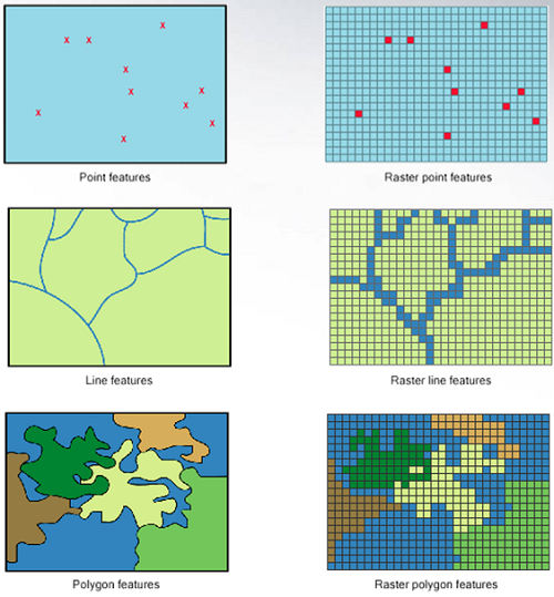
Shapefiles
Vector spatial data has multiple files associated with it. To read in you must provide the sub-folder and layer name.
library(rgdal) #read in shapefiles
library(sp) #working with spatial* class data

##download shapefile from drive
#url<-'https://drive.google.com/file/d/0B-TN-iTwt6b3aFlqSFVsTXVJT3M/view?usp=sharing' ##source of zip file
#download.file(url = url, destfile = 'data/BOUNDARY/CA_state')
#unzip('BOUNDARY/CA_state', exdir='BOUNDARY')##unzip shapefiles
cali<-readOGR('data/BOUNDARY/CA_state')

#capd_url<-'https://drive.google.com/file/d/0B-TN-iTwt6b3Z3VPaktBNTFUQUk/view?usp=sharing'
#download.file(url = capd_url, destfile = 'data/BOUNDARY/CAPD')
#unzip('BOUNDARY/CAPD', exdir='BOUNDARY')
CAPD<-readOGR(dsn='data/BOUNDARY/CPAD', layer='super_units')##CA protected areas
Spatial* objects
sp package
- SpatialPolygonDataFrame
- SpatialPointsDataFrame
- SpatialGridDataFrame
class(cali)
## [1] "SpatialPolygonsDataFrame"
## attr(,"package")
## [1] "sp"
cali@proj4string ##projection
## CRS arguments: +proj=longlat +ellps=WGS84 +no_defs
head(cali@data) ##attribute data
##   REGION DIVISION STATEFP  STATENS GEOID STUSPS       NAME LSAD MTFCC
## 0      4        9      06 01779778    06     CA California   00 G4000
##   FUNCSTAT        ALAND      AWATER    INTPTLAT     INTPTLON
## 0        A 403501101370 20466718403 +37.1551773 -119.5434183
Spatial* objects
SpatialPolygonDataFrame
plot(cali)

SpatialPointsDataFrame
Convert coordinate points to spatial* df
plants<-sp.df%>%
  filter(kingdom=='plant')

##convert lat/long coordinates to spdf
plant.spdf<-SpatialPointsDataFrame(coords=plants[,c('Long','Lat')],
                       data=plants, proj4string = CRS("+proj=longlat +ellps=WGS84 +no_defs"))##assign projection
summary(plant.spdf)
## Object of class SpatialPointsDataFrame
## Coordinates:
##            min        max
## Long -124.2415 -114.09480
## Lat    32.5596   55.19738
## Is projected: FALSE
## proj4string : [+proj=longlat +ellps=WGS84 +no_defs]
## Number of points: 3558
## Data attributes:
##                         name                  basisOfRecord
##  Dudleya cymosa           : 564   HUMAN_OBSERVATION  :1470
##  Opuntia basilaris        : 403   MACHINE_OBSERVATION:   0
##  Streptanthus glandulosus : 324   OBSERVATION        :   0
##  Arctostaphylos glandulosa: 225   PRESERVED_SPECIMEN :2077
##  Dudleya abramsii         : 192   UNKNOWN            :  11
##  Eriastrum densifolium    : 138
##  (Other)                  :1712
##       year          month             day           taxonkey
##  Min.   :2007   Min.   : 1.000   Min.   : 1.00   Min.   :2684012
##  1st Qu.:2009   1st Qu.: 4.000   1st Qu.: 9.00   1st Qu.:2985885
##  Median :2011   Median : 5.000   Median :16.00   Median :3041603
##  Mean   :2012   Mean   : 5.357   Mean   :16.14   Mean   :3606683
##  3rd Qu.:2015   3rd Qu.: 6.000   3rd Qu.:23.00   3rd Qu.:3188882
##  Max.   :2016   Max.   :12.000   Max.   :31.00   Max.   :9080971
##                                  NA's   :2
##       Long             Lat        Status
##  Min.   :-124.2   Min.   :32.56   E:2598
##  1st Qu.:-121.9   1st Qu.:34.20   T: 960
##  Median :-119.6   Median :36.42
##  Mean   :-119.4   Mean   :36.36
##  3rd Qu.:-116.8   3rd Qu.:38.24
##  Max.   :-114.1   Max.   :55.20
##
##                                                        Species.Listing.Name
##  Cactus, Bakersfield (Opuntia treleasei)                         : 403
##  Dudleya, marcescent (Dudleya cymosa ssp. marcescens)            : 282
##  Dudleya, Santa Monica Mountains (Dudleya cymosa ssp. ovatifolia): 282
##  Manzanita, Del Mar (Arctostaphylos glandulosa ssp. crassifolia) : 225
##  Jewelflower, Metcalf Canyon (Streptanthus albidus ssp. albidus) : 162
##  Jewelflower, Tiburon (Streptanthus niger)                       : 162
##  (Other)                                                         :2042
##    kingdom                 organism
##  animal:   0   Dudleya         : 761
##  plant :3558   Cactus          : 403
##                Jewelflower     : 326
##                Manzanita       : 278
##                Evening-primrose: 149
##                Woolly-star     : 138
##                (Other)         :1503
##                                    species             rank
##  Opuntia treleasei                     : 403   SPECIES   :1563
##  Dudleya cymosa  marcescens            : 282   SUBSPECIES:1995
##  Dudleya cymosa  ovatifolia            : 282
##  Arctostaphylos glandulosa  crassifolia: 225
##  Streptanthus albidus  albidus         : 162
##  Streptanthus niger                    : 162
##  (Other)                               :2042
##             class           date
##  Magnoliopsida :3308   Min.   :2007-01-29
##  Liliopsida    : 241   1st Qu.:2009-07-08
##  Pinopsida     :   9   Median :2011-08-16
##  Actinopterygii:   0   Mean   :2012-03-16
##  Amphibia      :   0   3rd Qu.:2015-04-01
##  Aves          :   0   Max.   :2016-10-04
##  (Other)       :   0   NA's   :2
When combining spatial objects it is critical that they have the same projection & resolution.
Subset Spatial* points
plot(plant.spdf)

Subset Spatial* points
subsets objects of spatial classes by other spatial objects
CA_occ<-plant.spdf[cali,] ##subset observations to those within CA

#plot(cali)
plot(CA_occ)

Spatial overlay
At the spatial locations of x, retrieve attributes of y:
#are species observed in protected areas? which ones?
pts.capd<-over(x = plant.spdf, y = CAPD, returnList=FALSE)
str(pts.capd)
## 'data.frame':    3558 obs. of  12 variables:
##  $ ACCESS_TYP: Factor w/ 4 levels "No Public Access",..: NA NA 2 2 NA 2 2 NA NA NA ...
##  $ PARK_NAME : Factor w/ 12798 levels "105th Street Pocket Park",..: NA NA 510 8670 NA 4435 4435 NA NA NA ...
##  $ PARK_URL  : Factor w/ 1465 levels "http://ahs.ausd.net/",..: NA NA NA 589 NA 1029 1029 NA NA NA ...
##  $ SUID_NMA  : Factor w/ 14715 levels "10131","10132",..: NA NA 13754 190 NA 665 665 NA NA NA ...
##  $ MNG_AG_ID : Factor w/ 1043 levels "100","1000","1001",..: NA NA 481 75 NA 509 509 NA NA NA ...
##  $ MNG_AGENCY: Factor w/ 1043 levels "Adelanto, City of",..: NA NA 104 962 NA 107 107 NA NA NA ...
##  $ MNG_AG_LEV: Factor w/ 8 levels "City","County",..: NA NA 8 3 NA 8 8 NA NA NA ...
##  $ MNG_AG_TYP: Factor w/ 33 levels "Airport District",..: NA NA 31 8 NA 31 31 NA NA NA ...
##  $ AGNCY_WEB : Factor w/ 947 levels "http://acfloodcontrol.org/",..: NA NA 947 544 NA 723 723 NA NA NA ...
##  $ LAYER     : Factor w/ 14 levels "California Department of Fish and Wildlife",..: NA NA 1 13 NA 2 2 NA NA NA ...
##  $ ACRES     : num  NA NA 14583 1203452 NA ...
##  $ LABEL_NAME: Factor w/ 12693 levels "105th Street PP",..: NA NA 510 8667 NA 4433 4433 NA NA NA ...
Returns row of CAPD@data for every coordinate in magnoliid.spdf
Look at observations, species richness across parks:
plant.spdf$PARK_NAME<-pts.capd$PARK_NAME

protected<-plant.spdf@data%>%
  left_join(CAPD@data[,c('PARK_NAME','ACRES','MNG_AGENCY')], by='PARK_NAME')%>%
  group_by(PARK_NAME)%>%
  summarize(sps_n = length(unique(name)), obs_n = length(name),
            total_acres = sum(ACRES),
            mgmt = paste(unique(MNG_AGENCY), collapse=', '))%>% #concatenate mng_agency
  mutate(sps_area = obs_n/log(total_acres))%>%
  arrange(desc(sps_n))
protected[1:6,]
## # A tibble: 6 × 6
##                                  PARK_NAME sps_n obs_n total_acres
##                                     <fctr> <int> <int>       <dbl>
## 1                                       NA   101  1239          NA
## 2                                      BLM    30  1295  3722850054
## 3           San Bernardino National Forest    18   357   240481077
## 4                Cleveland National Forest    10    76    32298974
## 5 Marin Municipal Water District Watershed     9   117     2196865
## 6                  Angeles National Forest     8   405    89122471
## # ... with 2 more variables: mgmt <chr>, sps_area <dbl>
San Bernardino National Forest
sbnf<-CAPD[CAPD$PARK_NAME == 'San Bernardino National Forest',]
rm(CAPD)

plot(sbnf, col = 'darkgreen')

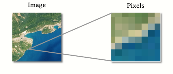
Raster data
PRISM climate
library(prism)
options(prism.path = "/Volumes/collnell/CAT/data/prism/prism_temp")
get_prism_normals(type = 'tmax', resolution = '800m', mon = 07, keepZip = TRUE)##July ma temperatures
##
  |
  |                                                                 |   0%
  |
  |=================================================================| 100%
PRISM climate
head(ls_prism_data(name=FALSE)) #all prism data files in working directory
##                                  files
## 1  PRISM_tmax_30yr_normal_4kmM2_07_bil
## 2 PRISM_tmax_30yr_normal_800mM2_07_bil
## 3   PRISM_tmax_stable_4kmM2_201007_bil
## 4   PRISM_tmax_stable_4kmM2_201107_bil
## 5   PRISM_tmax_stable_4kmM2_201207_bil
## 6   PRISM_tmax_stable_4kmM2_201307_bil
filein<-2 ##select corresponding row number
RS <- prism_stack(ls_prism_data()[filein,1]) ##raster file of data
proj4string(RS)<-CRS("+proj=longlat +ellps=WGS84 +towgs84=0,0,0,0,0,0,0 +units=m +no_defs") ##assign projection

filename<-paste0('PRISM_tmax_30yr_norm_07')
writeRaster(RS, filename=filename, overwrite=TRUE) ##save raster file
PRISM climate
See the PRISM tutorial for more on the PRISM package.
plot(RS, main='Max temperature (July) 30-year average')

Raster structure
tmax_norm<-raster(filename) ##read in raster (.tiff, .grd, asc)
tmax_norm@extent ##dimensions of the layer
## class       : Extent
## xmin        : -125.0208
## xmax        : -66.47917
## ymin        : 24.0625
## ymax        : 49.9375
tmax_norm@crs ##raster projection
## CRS arguments:
##  +proj=longlat +ellps=WGS84 +towgs84=0,0,0,0,0,0,0 +units=m
## +no_defs
#projectRaster() #to change projection
Crop raster by extent
sb.box<-extent(sbnf)
sb.box
## class       : Extent
## xmin        : -117.6525
## xmax        : -116.319
## ymin        : 33.49937
## ymax        : 34.3831
sb.norms<-crop(tmax_norm, sb.box)
plot(sb.norms)

Crop raster to polygon
norm.sbnf<-mask(sb.norms, sbnf)
norm.sbnf<-trim(norm.sbnf)

rm(tmax_norm)

plot(norm.sbnf, main="Average annual maximum temperature")
 ## Calculate temperature anomaly {.build}
Anomaly - deviation from normal or expected
Max temperature in 2050 under moderate emissions scenario
tmax_url<-'https://drive.google.com/file/d/0B-TN-iTwt6b3Z3JyM21KNUZidm8/view?usp=sharing'
download.file(url = tmax_url, destfile = 'data/CMIP5_NA/tmax_2050_a1b')
unzip('CMIP5_NA/tmax_2050_a1b', exdir='CMIP5_NA')
tmax_2050<-raster('data/climate/CMIP5_NA/tmax_2050_a1b.grd')
tamx_anom<-overlay(x = tmax_2050, y = norm.sbnf, fun=function(x,y){return(x-y)})
##C to F
tamx_anom@data@values<-tamx_anom@data@values*1.8+32
plot(tamx_anom, main='Projected max temp increase by 2050')

Extract values from raster
Polygon:
sb.anom<-extract(tamx_anom, sbnf, fun=mean, na.rm=TRUE, sp=TRUE)
sb.anom@data$layer ##what is the mean projected increase in high temps in SB nf?
## [1] 36.72586
Extract values from raster
Points:
sb.plants<-plant.spdf[sbnf,]##subset plant observations
sb.anom<-extract(tamx_anom, sb.plants, buffer=5, na.rm=TRUE, sp=TRUE)  ##sp adds to df

##which species will endure hottest heats?
heat<-sb.anom@data%>%group_by(name)%>%summarize(hot=mean(layer, na.rm=TRUE))%>%arrange(desc(hot))
heat
## # A tibble: 18 × 2
##                            name      hot
##                          <fctr>    <dbl>
## 1            Castilleja cinerea 39.44973
## 2              Poa atropurpurea 39.04857
## 3              Eremogone ursina 38.84712
## 4        Taraxacum californicum 38.78572
## 5               Physaria kingii 38.58729
## 6              Dudleya abramsii 37.34736
## 7             Cirsium scariosum 37.31629
## 8             Astragalus albens 37.14959
## 9                Carex lemmonii 36.83681
## 10    Arctostaphylos glandulosa 36.81242
## 11        Eriastrum densifolium 36.56150
## 12 Fremontodendron californicum 36.54928
## 13            Erigeron parishii 36.53058
## 14               Dudleya cymosa 36.35043
## 15            Opuntia basilaris 36.09442
## 16   Trichostema austromontanum 35.31437
## 17      Astragalus tricarinatus 35.18673
## 18        Dodecahema leptoceras 33.83153
Resources
dplyr cheatsheet: https://www.rstudio.com/wp-content/uploads/2015/02/data-wrangling-cheatsheet.pdf
CRAN task view: https://cran.r-project.org/web/views/Spatial.html
Spatial.ly: http://spatial.ly/r/
sf package: https://cran.r-project.org/web/packages/sf/vignettes/sf1.html