A Review of Nonlinear Time Series Models
Ran Wang
Contents
TAR: Threshold Autoregressive
SETAR (Self-Exciting Threshold Autoregressive)
SETAR (Self-Exciting Threshold Autoregressive)
SETAR (Self-Exciting Threshold Autoregressive)
SETAR (Self-Exciting Threshold Autoregressive)
SETAR (Self-Exciting Threshold Autoregressive)
SETAR (Self-Exciting Threshold Autoregressive)
Model Estimation: Tsay's Approach

SETAR (Self-Exciting Threshold Autoregressive)
SETAR (Self-Exciting Threshold Autoregressive)
STAR (Smooth Transition Autoregressive)
STAR (Smooth Transition Autoregressive)
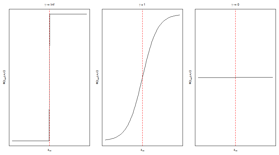
- 1 Logistic STAR:
\[ G(z_t)=\frac{1}{1+e^{-\gamma(z_t-c)}} \]
STAR (Smooth Transition Autoregressive)
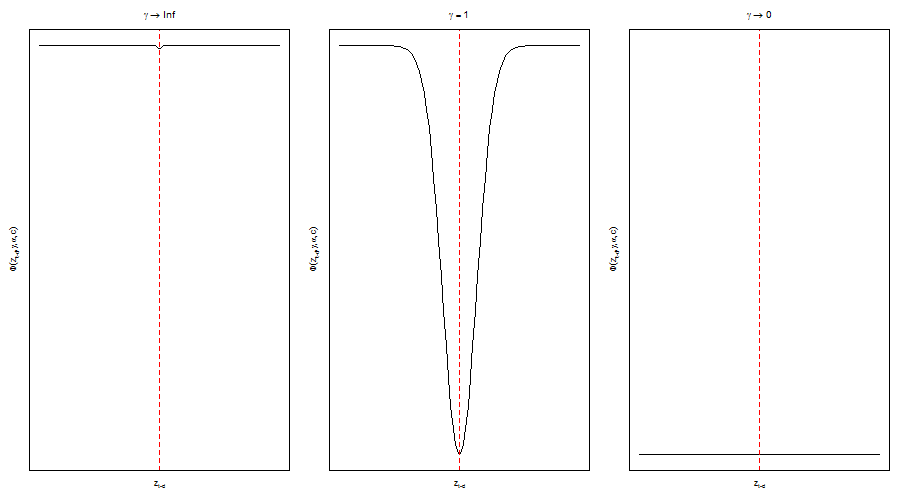
- 2 Exponential STAR:
\[ G(z_t)=1-e^{-\gamma(z_t-c)^2} \]