Slides: rpubs.com/RobinLovelace
Introduction
Course outline
- An introduction to R based on Collin Gillespie's Introduction to R (13:30 - 14:00)
- Practical: Working through the Introduction to R booklet (14:00 - 15:00)
- Demonstration of working with transport data in R (15:00 - 15:30)
- Practical: Working through R for Spatial Planning and Analysis (15:30 - 16:30)
- Additional practical: Do the question and answer challenges in the nclRintroduction package
- Advanced practical: reproducing the results in the stplanr-paper vignette.
Context
See the thesis-reproducible repo
One of the first maps I made for my thesis
What R can do - Propensity to Cycle Tool
See pct.bike
A bit about R
- Developed by statisticians Ross Ihaka and Robert Gentleman
- De-facto standard for advanced statistical analysis
- A programming language in its own right
- The power of the command line
- Used by an increasing number of organisations
Why R?
- Performace: stable, light and fast
- Support network
- documentation, community, developers
- Reproducibility
- anyone anywhere can reproduce results
- enables dissemination (RPubs, RMarkdown, .RPres) - this presentation is a .Rmd file!
- Versatility: unified solution to almost any numerical problem, graphical capabilities
- Ethics removes economic barrier to statistics, is open and democratic
R is up and coming
Source: r4stats
Source: r4stats.com
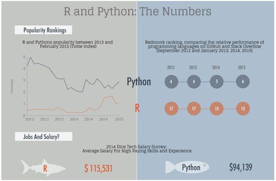
III - R vs Python
Source: kdnuggets

Source: Data Camp
IV - employment market
jobs
Source: revolution analytics
Visualisation
- R's visualisation capabilities have evolved over time
- Used to create plots in the best academic journals
- ggplot2 has revolutionised the visualisation of quantitative information in R, and (possibly) overall
- Thus there are different camps with different preferences when it comes to maps in R
Demonstration 1: The RStudio IDE
R as a giant calculator
5 * 5
1 + 4 * 5
4 * 5 ^ 2
sin(90)
sin(0.5 * pi)
Objects
a <- 1
b <- 2
c <- "c"
x_thingy <- 4
a + b
a * b
a + c
a / x_thingy
Adding and removing objects
ls()
## [1] "a" "b" "c" "x_thingy"
x <- x_thingy
rm(x_thingy)
x
## [1] 4
ls()
## [1] "a" "b" "c" "x"
Harmonograph example
- Complex outputs can be created with simple inputs
t <- 1:1000 / 10
x <- sin(t) * exp(t * - 0.01)
y <- sin(pi / 2 + t / 3) * exp(t * -0.01)
plot(x, y, "lines")
Practical 1: Getting used to RStudio and R
- Open RStudio and have a look around
- Create a new project
- Create a new R Script: pass code to the console with
Ctl-Enter - Use R as a calculator: what is:
\[ \pi * 9.15^2 \]
- Explore each of the 'panes'
- Find and write down some useful shortcuts (
Alt-Shift-Kon Windows/Linux)
Basic R functions and behaviour
Functions and objects
In R:
- Everything that exists is an object
- Everything that happens is a function
# Assignment of x
x <- 5
x
## [1] 5
# A trick to print x
(x <- 5)
(y <- x)
Functions
sin(x)
## [1] -0.9589243
exp(x)
## [1] 148.4132
factorial(x)
## [1] 120
sinx <- sin(x)
Assignment
x = 5 # the same as x <- 5
(x = x + 1)
## [1] 6
R is vector based
x <- c(1, 2, 5)
x
## [1] 1 2 5
x^2
## [1] 1 4 25
x + 2
## [1] 3 4 7
x + rev(x)
The classic programming way: verbose
x <- c(1, 2, 5)
for(i in x){
  print(i^2)
}
## [1] 1
## [1] 4
## [1] 25
Creating a new vector based on x
for(i in 1:length(x)){
  if(i == 1) x2 <- x[i]^2
  else x2 <- c(x2, x[i]^2)
}
x2
## [1] 1 4 25
Data types
R has a hierarchy of data classes, tending to the lowest:
- Binary
- Integer (numeric)
- Double (numeric)
- Character
Examples of data types
a <- TRUE
b <- 1:5
c <- pi
d <- "Hello Leeds"
class(a)
class(b)
class(c)
class(d)
Data type switching
ab <- c(a, b)
ab
## [1] 1 1 2 3 4 5
class(ab)
## [1] "integer"
Test on data types
class(c(a, b))
## [1] "integer"
class(c(a, c))
## [1] "numeric"
class(c(b, d))
## [1] "character"
Sequences
x <- 1:5
y <- 2:6
plot(x, y)
Sequences with seq
x <- seq(1,2, by = 0.2)
length(x)
## [1] 6
x <- seq(1, 2, length.out = 5)
length(x)
## [1] 5
Practical
- Work through Colin Gillespie's Introduction to R booklet
- Optional: install the R package
install.packages("drat")
drat::addRepo("rcourses")
install.packages("nclRintroduction", type="source")
library(nclRintroduction)
vignette(package = "nclRintroduction", "practical1")
Demo: Transport data with R
- Let's see how R can be used to analyse transport data:
library(stplanr)
## Loading required package: sp
data("routes_fast")
plot(routes_fast)
Practical - work through the tutorial
- See the source code here: https://github.com/ITSLeeds/SSPA/blob/master/r4transport.Rmd
- Experiment with the content
Using the 'nclRintroduction' package
if(!require(devtools))
  install.packages("devtools")
if(!require(nclRintroduction))
  devtools::install_github("rcourses/nclRintroduction", build_vignettes = T)
library(nclRintroduction)
vignette(package = "nclRintroduction")
Advanced challenge
- Reproduce the work documented in the
stplanr-papervignette
vignette("stplanr-paper")
- Experiment with the example datasets - can you make different versions of the plots?