Bioinformatics for Big Omics Data: Advanced data manipulation

width: 1440 height: 900 transition: none font-family: 'Helvetica' css: my_style.css author: Raphael Gottardo, PhD date: June 07, 2014

This work is licensed under a Creative Commons Attribution-ShareAlike 3.0 Unported License.

Here is a simple change

Motivation

Let's first turn on the cache for increased performance.

library(knitr)
# Set some global knitr options
opts_chunk$set(cache=TRUE)

R has pass-by-value semantics, which minimizes accidental side effects. However, this can become a major bottleneck when dealing with large datasets both in terms of memory and speed.
Working with data.frames in R can also be painful process in terms of writing code.
Fortunately, R provides some solution to this problems.

a <- rnorm(10^5)
gc()

##          used (Mb) gc trigger (Mb) max used (Mb)
## Ncells 250982 13.5     407500 21.8   350000 18.7
## Vcells 469179  3.6     905753  7.0   786432  6.0

b <- a
gc()

##          used (Mb) gc trigger (Mb) max used (Mb)
## Ncells 251113 13.5     467875   25   350000 18.7
## Vcells 469355  3.6     905753    7   786432  6.0

a[1] <- 0
gc()

##          used (Mb) gc trigger (Mb) max used (Mb)
## Ncells 251132 13.5     467875 25.0   350000 18.7
## Vcells 569386  4.4    1031040  7.9   786432  6.0

Overview

Here we will review three R packages that can be used to provide efficient data manipulation:

data.table: An package for efficient data storage and manipulation
RSQLite: Database Interface R driver for SQLite
sqldf: An R package for runing SQL statements on R data frames, optimized for convenience

Thank to Kevin Ushey (@kevin_ushey) for the data.table notes and Matt Dowle and Arunkumar Srinivasan for helpful comments.

What is data.table?

data.table is an R package that extends. R data.frames.

Under the hood, they are just data.frame's, with some extra 'stuff' added on. So, they're collections of equal-length vectors. Each vector can be of different type.

library(data.table)
dt <- data.table(x=1:3, y=c(4, 5, 6), z=letters[1:3])
dt

##    x y z
## 1: 1 4 a
## 2: 2 5 b
## 3: 3 6 c

class(dt)

## [1] "data.table" "data.frame"

The extra functionality offered by data.table allows us to modify, reshape, and merge data.tables much quicker than data.frames. See that data.table inherits from data.frame!

Note: The development version (v1.8.11) of data.table includes a lot of new features including melt and dcast methods

Installing data.table

stable CRAN release

install.packages("data.table")

latest bug-fixes + enhancements

install.packages("data.table", repos="http://R-forge.R-project.org")

What's different?

Most of your interactions with data.tables will be through the subset ([) operator, which behaves quite differently for data.tables. We'll examine a few of the common cases.

Visit this stackoverflow question for a summary of the differences between data.frames and data.tables.

Single element subsetting

library(data.table)
DF <- data.frame(x=1:3, y=4:6, z=7:9)
DT <- data.table(x=1:3, y=4:6, z=7:9)
DF[c(2,3)]

##   y z
## 1 4 7
## 2 5 8
## 3 6 9

DT[c(2,3)]

##    x y z
## 1: 2 5 8
## 2: 3 6 9

By default, single-element subsetting in data.tables refers to rows, rather than columns.

Row subsetting

library(data.table)
DF <- data.frame(x=1:3, y=4:6, z=7:9)
DT <- data.table(x=1:3, y=4:6, z=7:9)
DF[c(2,3), ]

##   x y z
## 2 2 5 8
## 3 3 6 9

DT[c(2,3), ]

##    x y z
## 1: 2 5 8
## 2: 3 6 9

Notice: row names are lost with data.tables. Otherwise, output is identical.

Column subsetting

library(data.table)
DF <- data.frame(x=1:3, y=4:6, z=7:9)
DT <- data.table(x=1:3, y=4:6, z=7:9)
DF[, c(2,3)]

##   y z
## 1 4 7
## 2 5 8
## 3 6 9

DT[, c(2,3)]

## [1] 2 3

DT[, c(2,3)] just returns c(2, 3). Why on earth is that?

The j expression

The subset operator is really a function, and data.table modifies it to behave differently.

Call the arguments we pass e.g. DT[i, j], or DT[i].

The second argument to [ is called the j expression, so-called because it's interpreted as an R expression. This is where most of the data.table magic happens.

j is an expression evaluated within the frame of the data.table, so it sees the column names of DT. Similarly for i.

First, let's remind ourselves what an R expression is.

Expressions

An expression is a collection of statements, enclosed in a block generated by braces {}.

## an expression with two statements
{
  x <- 1
  y <- 2
}
## the last statement in an expression is returned
k <- { print(10); 5 }

## [1] 10

print(k)

## [1] 5

The j expression (suite)

So, data.table does something special with the expression that you pass as j, the second argument, to the subsetting ([) operator.

The return type of the final statement in our expression determines the type of operation that will be performed.

In general, the output should either be a list of symbols, or a statement using :=.

We'll start by looking at the list of symbols as an output.

An example

When we simply provide a list to the j expression, we generate a new data.table as output, with operations as performed within the list call.

library(data.table)
DT <- data.table(x=1:5, y=1:5)
DT[, list(mean_x = mean(x), sum_y = sum(y), sumsq=sum(x^2+y^2))]

##    mean_x sum_y sumsq
## 1:      3    15   110

Notice how the symbols x and y are looked up within the data.table DT. No more writing DT$ everywhere!

Using :=

Using the := operator tells us we should assign columns by reference into the data.table DT:

library(data.table)
DT <- data.table(x=1:5)
DT[, y := x^2]

##    x  y
## 1: 1  1
## 2: 2  4
## 3: 3  9
## 4: 4 16
## 5: 5 25

print(DT)

##    x  y
## 1: 1  1
## 2: 2  4
## 3: 3  9
## 4: 4 16
## 5: 5 25

Using := (suite)

By default, data.tables are not copied on a direct assignment <-:

library(data.table)
DT <- data.table(x=1)
DT2 <- DT
DT[, y := 2]

##    x y
## 1: 1 2

DT2

##    x y
## 1: 1 2

Notice that DT2 has changed. This is something to be mindful of; if you want to explicitly copy a data.table do so with DT2 <- copy(DT).

A slightly more complicated example

library(data.table)
DT <- data.table(x=1:5, y=6:10, z=11:15)
DT[, m := log2( (x+1) / (y+1) )]

##    x  y  z       m
## 1: 1  6 11 -1.8074
## 2: 2  7 12 -1.4150
## 3: 3  8 13 -1.1699
## 4: 4  9 14 -1.0000
## 5: 5 10 15 -0.8745

print(DT)

##    x  y  z       m
## 1: 1  6 11 -1.8074
## 2: 2  7 12 -1.4150
## 3: 3  8 13 -1.1699
## 4: 4  9 14 -1.0000
## 5: 5 10 15 -0.8745

Using an expression in j

Note that the right-hand side of a := call can be an expression.

library(data.table)
DT <- data.table(x=1:5, y=6:10, z=11:15)
DT[, m := { tmp <- (x + 1) / (y + 1); log2(tmp) }]

##    x  y  z       m
## 1: 1  6 11 -1.8074
## 2: 2  7 12 -1.4150
## 3: 3  8 13 -1.1699
## 4: 4  9 14 -1.0000
## 5: 5 10 15 -0.8745

print(DT)

##    x  y  z       m
## 1: 1  6 11 -1.8074
## 2: 2  7 12 -1.4150
## 3: 3  8 13 -1.1699
## 4: 4  9 14 -1.0000
## 5: 5 10 15 -0.8745

Multiple returns from an expression in j

The left hand side of a := call can also be a character vector of names, for which the corresponding final statement in the j expression should be a list of the same length.

library(data.table)
DT <- data.table(x=1:5, y=6:10, z=11:15)
DT[, c('m', 'n') := { tmp <- (x + 1) / (y + 1); list( log2(tmp), log10(tmp) ) }]

##    x  y  z       m       n
## 1: 1  6 11 -1.8074 -0.5441
## 2: 2  7 12 -1.4150 -0.4260
## 3: 3  8 13 -1.1699 -0.3522
## 4: 4  9 14 -1.0000 -0.3010
## 5: 5 10 15 -0.8745 -0.2632

DT[, `:=`(a=x^2, b=y^2)]

##    x  y  z       m       n  a   b
## 1: 1  6 11 -1.8074 -0.5441  1  36
## 2: 2  7 12 -1.4150 -0.4260  4  49
## 3: 3  8 13 -1.1699 -0.3522  9  64
## 4: 4  9 14 -1.0000 -0.3010 16  81
## 5: 5 10 15 -0.8745 -0.2632 25 100

DT[, c("c","d"):=list(x^2, y^2)]

##    x  y  z       m       n  a   b  c   d
## 1: 1  6 11 -1.8074 -0.5441  1  36  1  36
## 2: 2  7 12 -1.4150 -0.4260  4  49  4  49
## 3: 3  8 13 -1.1699 -0.3522  9  64  9  64
## 4: 4  9 14 -1.0000 -0.3010 16  81 16  81
## 5: 5 10 15 -0.8745 -0.2632 25 100 25 100

The j expression revisited

So, we typically call j the j expression, but really, it's either:

An expression, or
A call to the function :=, for which the first argument is a set of names (vectors to update), and the second argument is an expression, with the final statement typically being a list of results to assign within the data.table.

As I said before, a := b is parsed by R as ":="(a, b), hence it looking somewhat like an operator.

quote(a := b)

## `:=`(a, b)

Why does it matter?

Whenever you sub-assign a data.frame, R is forced to copy the entire data.frame.

That is, whenever you write DF$x <- 1, DF["x"] <- 1, DF[["x"]] <- 1…

… R will make a copy of DF before assignment.

This is done in order to ensure any other symbols pointing at the same object do not get modified. This is a good thing for when we need to reason about the code we write, since, in general, we expect R to operate without side effects.

Unfortunately, it is prohibitively slow for large objects, and hence why := can be very useful.

Why does it matter?

library(data.table); library(microbenchmark)

## Error: there is no package called 'microbenchmark'

big_df <- data.frame(x=rnorm(1E6), y=sample(letters, 1E6, TRUE))
big_dt <- data.table(big_df)
microbenchmark( big_df$z <- 1, big_dt[, z := 1] )

## Error: could not find function "microbenchmark"

Once again, notice that := is actually a function, and z := 1 is parsed as ":="(z, 1).

Using by

We can also perform grouping like operations through the use of the by argument:

library(data.table)
DT <- data.table(x=1:5, y=6:10, gp=c('a', 'a', 'a', 'b', 'b'))
DT[, z := mean(x+y), by=gp]

##    x  y gp  z
## 1: 1  6  a  9
## 2: 2  7  a  9
## 3: 3  8  a  9
## 4: 4  9  b 14
## 5: 5 10  b 14

print(DT)

##    x  y gp  z
## 1: 1  6  a  9
## 2: 2  7  a  9
## 3: 3  8  a  9
## 4: 4  9  b 14
## 5: 5 10  b 14

Notice that since mean(x+y) returns a scalar (numeric vector of length 1), it is recycled to fill within each group.

Generating a new data.table

What if, rather than modifying the current data.table, we wanted to generate a new one?

library(data.table)
DT <- data.table(x=1:5, y=6:10, gp=c('a', 'a', 'a', 'b', 'b'))
DT[, list(z=mean(x + y)), by=gp]

##    gp  z
## 1:  a  9
## 2:  b 14

Notice that we retain one row for each unique group specified in the by argument, and only the by variables along-side our z variable are returned.

The j expression

A list

… returns a new data.table, potentially subset over groups in your by.

A := Call

… modifies that data.table in place, hence saving memory. Output is recycled if the by argument is used.

In general, our `j expression` is either:

an expression, with the final (or only) statement being a list of (named) arguments,
a call to the := function, with
- the first argument being names, and
- the second argument being an expression, for which the last statement is a list of the same length as the first argument.

Special variables

There are a number of special variables defined only within j, that allow us to do some neat things…

library(data.table)
data.table()[, ls(all=TRUE)]

## [1] ".GRP"  ".I"    ".iSD"  ".N"    ".SD"   ".xSD"  "print"

These variables allow us to infer a bit more about what's going on within the data.table calls, and also allow us to write more complicated j expressions.

Special variables

`.SD`

A data.table containing the subset of data for each group, excluding columns used in by.

`.BY`

A list containing a length 1 vector for each item in by.

`.N`

An integer, length 1, containing the number of rows in .SD.

`.I`

A vector of indices, holding the row locations from which .SD was pulled from the parent DT.

`.GRP`

A counter telling you which group you're working with (1st, 2nd, 3rd…)

Example usage of .N - Counts

Compute the counts, by group, using data.table…

set.seed(123); library(data.table); library(microbenchmark)

## Error: there is no package called 'microbenchmark'

DT <- data.table(x=sample(letters[1:3], 1E5, TRUE))
DT[, .N, by=x]

##    x     N
## 1: a 33387
## 2: c 33201
## 3: b 33412

table(DT$x)

## 
##     a     b     c 
## 33387 33412 33201

Example usage of .N - Counts

library(data.table)
library(microbenchmark)

## Error: there is no package called 'microbenchmark'

DT <- data.table(x=factor(sample(letters[1:3], 1E5, TRUE)))
microbenchmark( tbl=table(DT$x), DT=DT[, .N, by=x] )

## Error: could not find function "microbenchmark"

Example usage of .SD - lapply-type calls

library(data.table)
DT <- data.table(x=rnorm(10), y=rnorm(10), z=rnorm(10), id=letters[1:10])
DT[, lapply(.SD, mean), .SDcols=c('x', 'y', 'z')]

##         x        y       z
## 1: 0.2661 -0.09743 -0.3069

lapply(DT[,1:3, with=FALSE], mean)

## $x
## [1] 0.2661
## 
## $y
## [1] -0.09743
## 
## $z
## [1] -0.3069

Example usage of .SD - lapply-type calls

library(data.table); library(microbenchmark)

## Error: there is no package called 'microbenchmark'

DT <- data.table(x=rnorm(1E5), y=rnorm(1E5), z=sample(letters,1E5,replace=TRUE))
DT2 <- copy(DT)
setkey(DT2, "z")
microbenchmark(
  DT=DT[, lapply(.SD, mean), .SDcols=c('x', 'y'), by='z'],
  DT2=DT2[, lapply(.SD, mean), .SDcols=c('x', 'y'), by='z']
)

## Error: could not find function "microbenchmark"

setting a key can lead to faster grouping operations.

Keys

data.tables can be keyed, allowing for faster indexing and subsetting. Keys are also used for joins, as we'll see later.

library(data.table)
DT <- data.table(x=c('a', 'a', 'b', 'c', 'a'), y=rnorm(5))
setkey(DT, x)
DT['a'] ## grabs rows corresponding to 'a'

##    x        y
## 1: a  0.72342
## 2: a -1.13247
## 3: a  0.06334

Note that this does a binary search rather than a vector scan, which is much faster!

Key performance

library(data.table); library(microbenchmark)

## Error: there is no package called 'microbenchmark'

DF <- data.frame(key=sample(letters, 1E6, TRUE), x=rnorm(1E6))
DT <- data.table(DF)
setkey(DT, key)
identical( DT['a']$x, DF[ DF$key == 'a', ]$x )

## [1] TRUE

microbenchmark( DT=DT['a'], DF=DF[ DF$key == 'a', ], times=5 )

## Error: could not find function "microbenchmark"

Further reading: you can set multiple keys with setkeyv as well.

Joins

data.table comes with many kinds of joins, implements through the merge.data.table function, and also through the [ syntax as well. We'll focus on using merge.

library(data.table); library(microbenchmark)

## Error: there is no package called 'microbenchmark'

DT1 <- data.table(x=c('a', 'a', 'b', 'dt1'), y=1:4)
DT2 <- data.table(x=c('a', 'b', 'dt2'), z=5:7)
setkey(DT1, x)
setkey(DT2, x)
merge(DT1, DT2)

##    x y z
## 1: a 1 5
## 2: a 2 5
## 3: b 3 6

Overview of joins

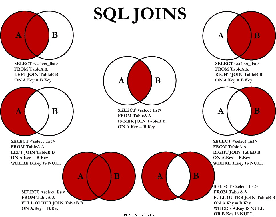
Here is a quick summary of SQL joins, applicable to data.table too.

(Source: http://www.codeproject.com)

SQL joins

A left join

library(data.table); library(microbenchmark)

## Error: there is no package called 'microbenchmark'

DT1 <- data.table(x=c('a', 'a', 'b', 'dt1'), y=1:4)
DT2 <- data.table(x=c('a', 'b', 'dt2'), z=5:7)
setkey(DT1, x)
setkey(DT2, x)
merge(DT1, DT2, all.x=TRUE)

##      x y  z
## 1:   a 1  5
## 2:   a 2  5
## 3:   b 3  6
## 4: dt1 4 NA

A right join

library(data.table); library(microbenchmark)

## Error: there is no package called 'microbenchmark'

DT1 <- data.table(x=c('a', 'a', 'b', 'dt1'), y=1:4)
DT2 <- data.table(x=c('a', 'b', 'dt2'), z=5:7)
setkey(DT1, x)
setkey(DT2, x)
merge(DT1, DT2, all.y=TRUE)

##      x  y z
## 1:   a  1 5
## 2:   a  2 5
## 3:   b  3 6
## 4: dt2 NA 7

An outer join

library(data.table); library(microbenchmark)

## Error: there is no package called 'microbenchmark'

DT1 <- data.table(x=c('a', 'a', 'b', 'dt1'), y=1:4)
DT2 <- data.table(x=c('a', 'b', 'dt2'), z=5:7)
setkey(DT1, x)
setkey(DT2, x)
merge(DT1, DT2, all=TRUE) ## outer join

##      x  y  z
## 1:   a  1  5
## 2:   a  2  5
## 3:   b  3  6
## 4: dt1  4 NA
## 5: dt2 NA  7

An inner join

library(data.table); library(microbenchmark)

## Error: there is no package called 'microbenchmark'

DT1 <- data.table(x=c('a', 'a', 'b', 'dt1'), y=1:4)
DT2 <- data.table(x=c('a', 'b', 'dt2'), z=5:7)
setkey(DT1, x)
setkey(DT2, x)
merge(DT1, DT2, all=FALSE) ## inner join

##    x y z
## 1: a 1 5
## 2: a 2 5
## 3: b 3 6

Speed example

library(data.table); library(microbenchmark)

## Error: there is no package called 'microbenchmark'

DT1 <- data.table(
  x=do.call(paste, expand.grid(letters, letters, letters, letters)), 
  y=rnorm(26^4)
)
DT2 <- DT1[ sample(1:nrow(DT1), 1E5), ]
setnames(DT2, c('x', 'z'))
DF1 <- as.data.frame(DT1)
DF2 <- as.data.frame(DT2)
setkey(DT1, x); setkey(DT2, x)
microbenchmark( DT=merge(DT1, DT2), DF=merge.data.frame(DF1, DF2), replications=5)

## Error: could not find function "microbenchmark"

Subset joins

We can also perform joins of two keyed data.tables using the [ operator. We perform right joins, so that e.g.

DT1[DT2]

is a right join of DT1 into DT2. These joins are typically a bit faster. Do note that the order of columns post-merge can be different, though.

Subset joins

library(data.table); library(microbenchmark)

## Error: there is no package called 'microbenchmark'

DT1 <- data.table(
  x=do.call(paste, expand.grid(letters, letters, letters, letters)), 
  y=rnorm(26^4)
)
DT2 <- DT1[ sample(1:nrow(DT1), 1E5), ]
setnames(DT2, c('x', 'z'))
setkey(DT1, x); setkey(DT2, x)
tmp1 <- DT2[DT1]
setcolorder(tmp1, c('x', 'y', 'z'))
tmp2 <- merge(DT1, DT2, all.x=TRUE)
setcolorder(tmp2, c('x', 'y', 'z'))
identical(tmp1, tmp2)

## [1] TRUE

Subset joins can be faster

library(data.table); library(microbenchmark)

## Error: there is no package called 'microbenchmark'

DT1 <- data.table(
  x=do.call(paste, expand.grid(letters, letters, letters, letters)), 
  y=rnorm(26^4)
)
DT2 <- DT1[ sample(1:nrow(DT1), 1E5), ]
setnames(DT2, c('x', 'z'))
setkey(DT1, x); setkey(DT2, x)
microbenchmark( bracket=DT1[DT2], merge=merge(DT1, DT2, all.y=TRUE), times=5 )

## Error: could not find function "microbenchmark"

Subset joins and the j-expression

More importantly they can be used the j-expression simultaneously, which can be very convenient.

DT1 <- data.table(x=1:5, y=6:10, z=11:15, key="x")
DT2 <- data.table(x=2L, y=7, w=1L, key="x")
# 1) subset only essential/necessary cols
DT1[DT2, list(z)]

##    x  z
## 1: 2 12

# 2) create new col
# i.y refer's to DT2's y col
DT1[DT2, list(newcol = y > i.y)]

##    x newcol
## 1: 2  FALSE

# 3) also assign by reference with `:=`
DT1[DT2, newcol := z-w]

##    x  y  z newcol
## 1: 1  6 11     NA
## 2: 2  7 12     11
## 3: 3  8 13     NA
## 4: 4  9 14     NA
## 5: 5 10 15     NA

data.table and SQL

We can understand the usage of [ as SQL statements. From FAQ 2.16:

data.table Argument	SQL Statement
i	WHERE
j	SELECT
:=	UPDATE
by	GROUP BY
i	ORDER BY (in compound syntax)
i	HAVING (in compound syntax)

Compound syntax refers to multiple subsetting calls, and generally isn't necessary until you really feel like a data.table expert:

DT[where,select|update,group by][having][order by][ ]...[ ]

data.table and SQL - Joins

Here is a quick summary table of joins in data.table.

SQL	data.table
LEFT JOIN	x[y]
RIGHT JOIN	y[x]
INNER JOIN	x[y, nomatch=0]
OUTER JOIN	merge(x,y,all=TRUE)

data.table and SQL

It's worth noting that I really mean it when I say that data.table is like an in-memory data base. It will even perform some basic query optimization!

library(data.table)
options(datatable.verbose=TRUE)
DT <- data.table(x=1:5, y=1:5, z=1:5, a=c('a', 'a', 'b', 'b', 'c'))
DT[, lapply(.SD, mean), by=a]

## Finding groups (bysameorder=FALSE) ... done in 0secs. bysameorder=TRUE and o__ is length 0
## lapply optimization changed j from 'lapply(.SD, mean)' to 'list(mean(x), mean(y), mean(z))'
## GForce optimized j to 'list(gmean(x), gmean(y), gmean(z))'

##    a   x   y   z
## 1: a 1.5 1.5 1.5
## 2: b 3.5 3.5 3.5
## 3: c 5.0 5.0 5.0

options(datatable.verbose=FALSE)

Some thoughts

The primary use of data.table is for efficient and elegant data manipulation including aggregation and joins.

library(data.table); library(microbenchmark)

## Error: there is no package called 'microbenchmark'

DT <- data.table(gp1=sample(letters, 1E6, TRUE), gp2=sample(LETTERS, 1E6, TRUE), y=rnorm(1E6))
microbenchmark( times=5,
  DT=DT[, mean(y), by=list(gp1, gp2)],
  DF=with(DT, tapply(y, paste(gp1, gp2), mean)))

## Error: could not find function "microbenchmark"

Unlike “split-apply-combine” approaches such as plyr, data is never split in data.table! data.table applies the function to each subset recursively (in C for speed). This keeps the memory footprint low - which is very essential for “big data”.

Other interesting convenience functions

like

DT = data.table(Name=c("Mary","George","Martha"), Salary=c(2,3,4))
# Use regular expressions
DT[Name %like% "^Mar"]

##      Name Salary
## 1:   Mary      2
## 2: Martha      4

set* functions set, setattr, setnames, setcolorder, setkey, setkeyv

setcolorder(DT, c("Salary", "Name"))
DT

##    Salary   Name
## 1:      2   Mary
## 2:      3 George
## 3:      4 Martha

DT[, (myvar):=NULL] remove a column

DT[,Name:=NULL]

##    Salary
## 1:      2
## 2:      3
## 3:      4

Bonuses: fread

data.table also comes with fread, a file reader much, much better than read.table or read.csv:

library(data.table); library(microbenchmark)

## Error: there is no package called 'microbenchmark'

big_df <- data.frame(x=rnorm(1E6), y=rnorm(1E6))
file <- tempfile()
write.table(big_df, file=file, row.names=FALSE, col.names=TRUE, sep="\t", quote=FALSE)
microbenchmark( fread=fread(file), r.t=read.table(file, header=TRUE, sep="\t"), times=1 )

## Error: could not find function "microbenchmark"

unlink(file)

Bonuses: rbindlist

Use this function to rbind a list of data.frames, data.tables or lists:

library(data.table); library(microbenchmark)

## Error: there is no package called 'microbenchmark'

dfs <- replicate(100, data.frame(x=rnorm(1E4), y=rnorm(1E4)), simplify=FALSE)
all.equal( rbindlist(dfs), data.table(do.call(rbind, dfs)) )

## [1] TRUE

microbenchmark( DT=rbindlist(dfs), DF=do.call(rbind, dfs), times=5 )

## Error: could not find function "microbenchmark"

Summary

To quote Matt Dowle

data.table builds on base R functionality to reduce 2 types of time :

programming time (easier to write, read, debug and maintain)
compute time

It has always been that way around, 1 before 2. The main benefit is the syntax: combining where, select|update and 'by' into one query without having to string along a sequence of isolated function calls. Reduced function calls. Reduced variable name repetition. Easier to understand.

Learning More

Read some of the [data.table] tagged questions on StackOverflow
Read through the data.table FAQ, which is surprisingly well-written and comprehensive.
Experiment!

Databases and the Structured Query Language (SQL)

A database is an organized collection of datasets (tables).
A database management system (DBMS) is a software system designed to allow the definition, creation, querying, update, and administration of databases.
Well-known DBMSs include MySQL, PostgreSQL, SQLite, Microsoft SQL Server, Oracle, etc.
Relational DBMSs (RDBMs) store data in a set of related tables
Most RDBMs use some form of the Structured Query Language (SQL)

Why do we even need databases?

The Structured Query Language (SQL)

Although SQL is an ANSI (American National Standards Institute) standard, there are different flavors of the SQL language.

The data in RDBMS is stored in database objects called tables.

A table is a collection of related data entries and it consists of columns and rows.

Here we will use SQLite, which is a self contained relational database management system. In contrast to other database management systems, SQLite is not a separate process that is accessed from the client application (e.g. MySQL, PostgreSQL).

Using RSQLite

Here we will make use of the Bioconductor project to load and use an SQLite database.

# You only need to run this once
source("http://bioconductor.org/biocLite.R")
biocLite(c("org.Hs.eg.db"))

# Now we can use the org.Hs.eg.db to load a database
library(org.Hs.eg.db)

## Error: there is no package called 'org.Hs.eg.db'

# Create a connection
Hs_con <- org.Hs.eg_dbconn()

## Error: could not find function "org.Hs.eg_dbconn"

# List tables
head(dbListTables(Hs_con))

## Error: could not find function "dbListTables"

# Or using an SQLite command (NOTE: This is specific to SQLite)
head(dbGetQuery(Hs_con, "SELECT name FROM sqlite_master WHERE type='table' ORDER BY name;"))

## Error: could not find function "dbGetQuery"

Using RSQLite (suite)

# What columns are available?
dbListFields(Hs_con, "gene_info")

## Error: could not find function "dbListFields"

dbListFields(Hs_con, "alias")

## Error: could not find function "dbListFields"

# Or using SQLite
# dbGetQuery(Hs_con, "PRAGMA table_info('gene_info');")

gc()

##            used (Mb) gc trigger  (Mb) max used  (Mb)
## Ncells   866997 46.4    1368491  73.1  1368491  73.1
## Vcells 12306957 93.9   32936871 251.3 32904616 251.1

alias <- dbGetQuery(Hs_con, "SELECT * FROM alias;")

## Error: could not find function "dbGetQuery"

gc()

##            used (Mb) gc trigger  (Mb) max used  (Mb)
## Ncells   866988 46.4    1368491  73.1  1368491  73.1
## Vcells 12306945 93.9   32936871 251.3 32904616 251.1

gene_info <- dbGetQuery(Hs_con, "SELECT * FROM gene_info;")

## Error: could not find function "dbGetQuery"

chromosomes <- dbGetQuery(Hs_con, "SELECT * FROM chromosomes;")

## Error: could not find function "dbGetQuery"

CD154_df <- dbGetQuery(Hs_con, "SELECT * FROM alias a JOIN gene_info g ON g._id = a._id WHERE a.alias_symbol LIKE 'CD154';")

## Error: could not find function "dbGetQuery"

gc()

##            used (Mb) gc trigger  (Mb) max used  (Mb)
## Ncells   866969 46.4    1368491  73.1  1368491  73.1
## Vcells 12306982 93.9   32936871 251.3 32904616 251.1

CD40LG_alias_df <- dbGetQuery(Hs_con, "SELECT * FROM alias a JOIN gene_info g ON g._id = a._id WHERE g.symbol LIKE 'CD40LG';")

## Error: could not find function "dbGetQuery"

gc()

##            used (Mb) gc trigger  (Mb) max used  (Mb)
## Ncells   866989 46.4    1368491  73.1  1368491  73.1
## Vcells 12307014 93.9   32936871 251.3 32904616 251.1

Some SQL Commands

SELECT

The SELECT is used to query the database and retrieve selected data that match the specific criteria that you specify:

SELECT column1 [, column2, …] FROM tablename WHERE condition

ORDER BY

ORDER BY clause can order column name in either ascending (ASC) or descending (DESC) order.

JOIN

There are times when we need to collate data from two or more tables. As with data.tables we can use LEFT/RIGHT/INNER JOINS

GROUP BY

The GROUP BY was added to SQL so that aggregate functions could return a result grouped by column values.

SELECT col_name, function (col_name) FROM table_name GROUP BY col_name

A “GROUP BY” example

dbGetQuery(Hs_con, "SELECT c.chromosome, COUNT(g.gene_name) AS count FROM chromosomes c JOIN gene_info g ON g._id = c._id WHERE c.chromosome IN (1,2,3,4,'X') GROUP BY c.chromosome ORDER BY count;")

## Error: could not find function "dbGetQuery"

Some more SQL commands

Some other SQL statements that might be of used to you:

CREATE TABLE

The CREATE TABLE statement is used to create a new table.

DELETE

The DELETE command can be used to remove a record(s) from a table.

DROP

To remove an entire table from the database use the DROP command.

CREATE VIEW

A view is a virtual table that is a result of SQL SELECT statement. A view contains fields from one or more real tables in the database. This virtual table can then be queried as if it were a real table.

Creating your own SQLite database in R

db <- dbConnect(SQLite(), dbname="./Data/SDY61/SDY61.sqlite")

## Error: could not find function "dbConnect"

dbWriteTable(conn = db, name = "hai", value = "./Data/SDY61/hai_result.txt", row.names = FALSE, header = TRUE, sep="\t")

## Error: could not find function "dbWriteTable"

dbWriteTable(conn = db, name = "cohort", value = "./Data/SDY61/arm_or_cohort.txt", row.names = FALSE, header = TRUE, sep="\t")

## Error: could not find function "dbWriteTable"

Creating your own SQLite database in R (suite)

dbListFields(db, "hai")

## Error: could not find function "dbListFields"

dbListFields(db, "cohort")

## Error: could not find function "dbListFields"

res <- dbGetQuery(db, "SELECT STUDY_TIME_COLLECTED, cohort.DESCRIPTION, MAX(VALUE_REPORTED) AS max_value FROM hai JOIN cohort ON hai.ARM_ACCESSION = cohort.ARM_ACCESSION WHERE cohort.DESCRIPTION LIKE '%TIV%' GROUP BY BIOSAMPLE_ACCESSION;")

## Error: could not find function "dbGetQuery"

head(res)

## Error: object 'res' not found

Using data.table to perform the same operations

# Read the tables using fread
hai <- fread("./Data/SDY61/hai_result.txt")

## Error: File is empty:
## /var/folders/61/gxr0r_bn11d99375_xbmvjzc0000gn/T//RtmplLzn55/file1727641b3d558

cohort <- fread("./Data/SDY61/arm_or_cohort.txt")

## Error: File is empty:
## /var/folders/61/gxr0r_bn11d99375_xbmvjzc0000gn/T//RtmplLzn55/file1727657ba61b

## Set keys before joining
setkey(hai, "ARM_ACCESSION")

## Error: object 'hai' not found

setkey(cohort, "ARM_ACCESSION")

## Error: object 'cohort' not found

## Inner join
dt_joined <- cohort[hai, nomatch=0]

## Error: object 'cohort' not found

## Summarize values
head(dt_joined[DESCRIPTION %like% "TIV", list(max_value=max(VALUE_REPORTED)), by="BIOSAMPLE_ACCESSION,STUDY_TIME_COLLECTED"])

## Error: object 'dt_joined' not found

The sqldf package

Sometimes it can be convenient to use SQL statements on dataframes. This is exactly what the sqldf package does.

library(sqldf)
data(iris)
sqldf("select * from iris limit 5")
sqldf("select count(*) from iris")
sqldf("select Species, count(*) from iris group by Species")

The sqldf package can even provide increased speed over pure R operations.

Summary

R base data.frames are convenient but often not adapted to large dataset manipulation (e.g. genomics).
Thankfully, there are good alternatives. My recommendtion is:
- Use data.table for your day-to-day operations
- When you have many tables and a complex schema, use sqlite.

Note: There many other R packages for “big data” such the bigmemory suite, biglm, ff, RNetcdf, rhdf5, etc.

Bioinformatics for Big Omics Data: Advanced data manipulation

Here is a simple change

Motivation

Overview

What is data.table?

Installing data.table

What's different?

Single element subsetting

Row subsetting

Column subsetting

The j expression

Expressions

The j expression (suite)

An example

Using :=

Using := (suite)

A slightly more complicated example

Using an expression in j

Multiple returns from an expression in j

The j expression revisited

Why does it matter?

Why does it matter?

Using by

Generating a new data.table

The j expression

In general, our j expression is either:

Special variables

Special variables

.SD

.BY

.N

.I

.GRP

Example usage of .N - Counts

Example usage of .N - Counts

Example usage of .SD - lapply-type calls

Example usage of .SD - lapply-type calls

Keys

Key performance

Joins

Overview of joins

A left join

A right join

An outer join

An inner join

Speed example

Subset joins

Subset joins

Subset joins can be faster

Subset joins and the j-expression

data.table and SQL

data.table and SQL - Joins

data.table and SQL

Some thoughts

Other interesting convenience functions

Bonuses: fread

Bonuses: rbindlist

Summary

Learning More

Databases and the Structured Query Language (SQL)

The Structured Query Language (SQL)

Using RSQLite

Using RSQLite (suite)

Some SQL Commands

SELECT

ORDER BY

JOIN

GROUP BY

A “GROUP BY” example

Some more SQL commands

CREATE TABLE

DELETE

DROP

CREATE VIEW

Creating your own SQLite database in R

Creating your own SQLite database in R (suite)

Using data.table to perform the same operations

The sqldf package

Summary

In general, our `j expression` is either:

`.SD`

`.BY`

`.N`

`.I`

`.GRP`