This document pertains to load data from MySql Database into MongoDB. When possible this will be done using R code. The following packages will be used:
RMySQL rmongodb rjson
The mongod executable should be running in the background.
## Warning: package 'RMySQL' was built under R version 3.2.4## Loading required package: DBI## Warning: package 'rmongodb' was built under R version 3.2.5For the purpose of this exercise, we will use the flights data base already loaded into MySQL on localHost. We will assume that similar environment is available.
First, we will connect to MySQL database and retrieve the data using the RMySQL package. The connection parameters should be changed if the environment available is different.
#Connect to MySQL database

flights_db_mysql <- dbConnect(MySQL(), user="root", password="admin",
                                       dbname="flights", host="localhost")
Then we will run queries to retrieve the data and store it. For the flights table, the data could not be loaded using the method from rmongodb and the mongoimport function will be used. To this effect a .csv file will be created. The path where this file is stored should be udpated to reproduce the results.
# .csv path for flights table

path_csv <- "C:/Users/vbrio/Documents/Cuny/DATA_607/project4/flights.csv"

airlines <- dbGetQuery(flights_db_mysql, "SELECT * FROM flights.airlines;")
airports <- dbGetQuery(flights_db_mysql, "SELECT * FROM flights.airports;")
weather <- dbGetQuery(flights_db_mysql, "SELECT * FROM flights.weather;")
planes <- dbGetQuery(flights_db_mysql, "SELECT * FROM flights.planes;")
flights <- dbGetQuery(flights_db_mysql, "SELECT * FROM flights.flights;")

write.csv(flights, file = path_csv)
Checking some elements of the data. Also, the .csv file is created with a extra column containing the record number. This column should be removed from the .csv file.
class(airports)## [1] "data.frame"class(airlines)## [1] "data.frame"class(weather)## [1] "data.frame"class(planes)## [1] "data.frame"class(flights)## [1] "data.frame"airlines[1:5, ] ## carrier name
## 1 9E Endeavor Air Inc.\r
## 2 AA American Airlines Inc.\r
## 3 AS Alaska Airlines Inc.\r
## 4 B6 JetBlue Airways\r
## 5 DL Delta Air Lines Inc.\rairports[1:5, ]## faa name lat lon alt tz dst
## 1 04G Lansdowne Airport 41.13047 -80.61958 1044 -5 A
## 2 06A Moton Field Municipal Airport 32.46057 -85.68003 264 -5 A
## 3 06C Schaumburg Regional 41.98934 -88.10124 801 -6 A
## 4 06N Randall Airport 41.43191 -74.39156 523 -5 A
## 5 09J Jekyll Island Airport 31.07447 -81.42778 11 -4 Aweather[1:5, ]## origin year month day hour temp dewp humid wind_dir wind_speed
## 1 EWR 2013 1 1 0 37.04 21.92 53.97 230 10.35702
## 2 EWR 2013 1 1 1 37.04 21.92 53.97 230 13.80936
## 3 EWR 2013 1 1 2 37.94 21.92 52.09 230 12.65858
## 4 EWR 2013 1 1 3 37.94 23.00 54.51 230 13.80936
## 5 EWR 2013 1 1 4 37.94 24.08 57.04 240 14.96014
## wind_gust precip pressure visib
## 1 11.91865 0 1013.9 10
## 2 15.89154 0 1013.0 10
## 3 14.56724 0 1012.6 10
## 4 15.89154 0 1012.7 10
## 5 17.21583 0 1012.8 10planes[1:5, ]## tailnum year type manufacturer model engines
## 1 N10156 2004 Fixed wing multi engine EMBRAER EMB-145XR 2
## 2 N102UW 1998 Fixed wing multi engine AIRBUS INDUSTRIE A320-214 2
## 3 N103US 1999 Fixed wing multi engine AIRBUS INDUSTRIE A320-214 2
## 4 N104UW 1999 Fixed wing multi engine AIRBUS INDUSTRIE A320-214 2
## 5 N10575 2002 Fixed wing multi engine EMBRAER EMB-145LR 2
## seats speed engine
## 1 55 NA Turbo-fan
## 2 182 NA Turbo-fan
## 3 182 NA Turbo-fan
## 4 182 NA Turbo-fan
## 5 55 NA Turbo-fanflights[1:5, ]## year month day dep_time dep_delay arr_time arr_delay carrier tailnum
## 1 2013 1 1 517 2 830 11 UA N14228
## 2 2013 1 1 533 4 850 20 UA N24211
## 3 2013 1 1 542 2 923 33 AA N619AA
## 4 2013 1 1 544 -1 1004 -18 B6 N804JB
## 5 2013 1 1 554 -6 812 -25 DL N668DN
## flight origin dest air_time distance hour minute
## 1 1545 EWR IAH 227 1400 5 17
## 2 1714 LGA IAH 227 1416 5 33
## 3 1141 JFK MIA 160 1089 5 42
## 4 725 JFK BQN 183 1576 5 44
## 5 461 LGA ATL 116 762 6 54nrow(airlines)## [1] 16nrow(airports)## [1] 1397nrow(weather)## [1] 8719nrow(planes)## [1] 3322nrow(flights)## [1] 336776We will now connect to Mongodb database and we will load the data from the airlines, airports, weather, and planes tables. For the flight table the data will be imported from mongo shell by the mongoimport command. We were encoutering memory problem with the method outline below.
######################################################
#Connect to Mongodb database
# connect to mongodb running in background on localhost

# Please note, flights_m, was created using mongo shell
#######################################################
mongo <- mongo.create()
mongo.is.connected(mongo)
## [1] TRUEdb <- "flights_m"
mairlines <- "flights_m.airlines"
mairports <- "flights_m.airports"
mweather <- "flights_m.weather"
mplanes <- "flights_m.planes"
mflights <-"flights_m.flights"
mongo.get.database.collections(mongo, db)## character(0)The data must be converted to bjson format prior to being inserted into Mongodb database.
# convert airports l to bson format
airlines_lbson <- lapply(split(airlines, 1:nrow(airlines)), function(x) mongo.bson.from.JSON(toJSON(x)))
airports_lbson <- lapply(split(airports, 1:nrow(airports)), function(x) mongo.bson.from.JSON(toJSON(x)))
weather_lbson <- lapply(split(weather, 1:nrow(weather)), function(x) mongo.bson.from.JSON(toJSON(x)))
planes_lbson <- lapply(split(planes, 1:nrow(planes)), function(x) mongo.bson.from.JSON(toJSON(x)))
#flights_lbson <- lapply(split(flights, 1:nrow(flights)), function(x) mongo.bson.from.JSON(toJSON(x)))
# flights table is not being loaded.  Will write to .csv and load with dbmongo import.
We now inser the data into mongodb, the the collection already exists, we will remove it as to not duplicate the data.
if(mongo.count(mongo,mairlines) != 0){
  mongo.remove(mongo, mairlines, criteria = mongo.bson.empty())
}
## [1] TRUEmongo.insert.batch(mongo, mairlines, airlines_lbson)## [1] TRUEif(mongo.count(mongo,mairports) != 0){
mongo.remove(mongo, mairports, criteria = mongo.bson.empty())
}## [1] TRUEmongo.insert.batch(mongo, mairports, airports_lbson)## [1] TRUEif(mongo.count(mongo,mweather) != 0){
mongo.remove(mongo, mweather, criteria = mongo.bson.empty())
}## [1] TRUEmongo.insert.batch(mongo, mweather, weather_lbson)## [1] TRUEif(mongo.count(mongo,mplanes) != 0){
mongo.remove(mongo, mplanes, criteria = mongo.bson.empty())
}## [1] TRUEmongo.insert.batch(mongo, mplanes, planes_lbson)## [1] TRUEFor the flights table, the data will be inserted directly using the mongoimport command.
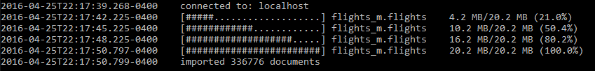
https://raw.githubusercontent.com/vbriot28/datascienceCUNY_607/master/import_command.PNG
The results we objtained:
https://raw.githubusercontent.com/vbriot28/datascienceCUNY_607/master/import_commnad_result.PNG
We will now compare the count between the set of records.
mongo.count(mongo, mairlines)## [1] 16mongo.count(mongo, mairports)## [1] 1397mongo.count(mongo, mweather)## [1] 8719mongo.count(mongo, mplanes)## [1] 3322mongo.count(mongo, mflights)## [1] 336776mysql_count <- c(nrow(airlines), nrow(airports), nrow(weather), nrow(planes), nrow(flights))
mongodb_count <- c(mongo.count(mongo, mairlines), mongo.count(mongo, mairports), mongo.count(mongo, mweather), mongo.count(mongo, mplanes),
mongo.count(mongo, mflights))
mysql_count == mongodb_count## [1] TRUE TRUE TRUE TRUE TRUEWe will now run a query on one of the table using both SQL and Mongodb. We will present the data into data frame. The query will select the record from the “weather” table for which origin = “JFK”.
mongo_l <- mongo.find.all(mongo, mweather, '{"origin" : "JFK"}')

class(mongo_l)
## [1] "list"mongo_df<-as.data.frame(do.call(rbind.data.frame, mongo_l))
class(mongo_df)## [1] "data.frame"sql_df <- dbGetQuery(flights_db_mysql, "SELECT * FROM flights.weather where origin = 'JFK';")
sql_df## origin year month day hour temp dewp humid wind_dir wind_speed
## 1 JFK 2013 2 18 4 17.96 -0.94 42.69 290 29.92028
## 2 JFK 2013 2 20 19 32.00 8.06 36.03 280 26.46794
## 3 JFK 2013 7 2 11 71.60 69.80 94.06 180 11.50780
## 4 JFK 2013 7 2 13 71.60 69.80 94.06 190 10.35702
## 5 JFK 2013 7 31 6 71.06 55.04 56.93 320 8.05546
## 6 JFK 2013 9 2 20 75.20 73.40 94.14 200 4.60312
## 7 JFK 2013 10 23 10 48.92 39.02 68.51 60 4.60312
## 8 JFK 2013 10 23 11 48.92 39.02 68.51 40 4.60312
## 9 JFK 2013 12 17 5 26.96 10.94 50.34 40 4.60312
## wind_gust precip pressure visib
## 1 34.431660 0 1016.2 10
## 2 30.458776 0 1011.2 10
## 3 13.242946 0 NA 0
## 4 11.918651 0 NA 1
## 5 9.270062 0 1020.4 10
## 6 5.297178 0 NA 4
## 7 5.297178 0 1008.1 10
## 8 5.297178 0 1008.5 10
## 9 5.297178 0 1023.9 10dim(mongo_df)## [1] 9 15dim(sql_df)## [1] 9 14mongo_df[,2:15] == sql_df## origin year month day hour temp dewp humid wind_dir wind_speed
## 2 TRUE TRUE TRUE TRUE TRUE TRUE TRUE TRUE TRUE TRUE
## 21 TRUE TRUE TRUE TRUE TRUE TRUE TRUE TRUE TRUE TRUE
## 3 TRUE TRUE TRUE TRUE TRUE TRUE TRUE TRUE TRUE TRUE
## 4 TRUE TRUE TRUE TRUE TRUE TRUE TRUE TRUE TRUE TRUE
## 5 TRUE TRUE TRUE TRUE TRUE TRUE TRUE TRUE TRUE TRUE
## 6 TRUE TRUE TRUE TRUE TRUE TRUE TRUE TRUE TRUE TRUE
## 7 TRUE TRUE TRUE TRUE TRUE TRUE TRUE TRUE TRUE TRUE
## 8 TRUE TRUE TRUE TRUE TRUE TRUE TRUE TRUE TRUE TRUE
## 9 TRUE TRUE TRUE TRUE TRUE TRUE TRUE TRUE TRUE TRUE
## wind_gust precip pressure visib
## 2 TRUE TRUE TRUE TRUE
## 21 TRUE TRUE TRUE TRUE
## 3 TRUE TRUE NA TRUE
## 4 TRUE TRUE NA TRUE
## 5 TRUE TRUE TRUE TRUE
## 6 TRUE TRUE NA TRUE
## 7 TRUE TRUE TRUE TRUE
## 8 TRUE TRUE TRUE TRUE
## 9 TRUE TRUE TRUE TRUEmongo_df$pressure## [1] 1016.2 1011.2 NA NA 1020.4 NA 1008.1 1008.5 1023.9
## Levels: 1008.1 1008.5 1011.2 1016.2 1020.4 1023.9 NAsql_df$pressure## [1] 1016.2 1011.2 NA NA 1020.4 NA 1008.1 1008.5 1023.9The ‘NA’ results we obtain in the dataframe to dataframe comparison are due to NA value in the pressure column. These values are ‘NA’ in both data sets, the one extracting from sql and the one extracting from mongodb.
In conclusion, with the rmongodb package, db opertion can be executed from R directly. However, the advantage of using Mongodb as a data base is to have a dynamic schema data base that can store large amount of data. We would anticipate that any work in R would be done in subset of original data set. The most efficient way of loading the data would be using the command provided by the database package. We would expect that a subset of the data would be loaded in R for transformation and analysis.
An interest video on rmongodb can be found here…
https://www.youtube.com/watch?v=GWZdFFYrR4I