Plot with Lakers’ Court and Regular Season vs. Playoffs
Mike
April 17, 2016
1. Plot with the Lakers’ Court:
I found this amazing Laker’s home court image and decided to use it for plots Lakers’ Court
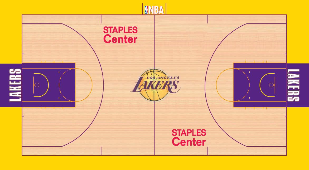
I rotated it and it is stored in my Github repo: Court Rotated
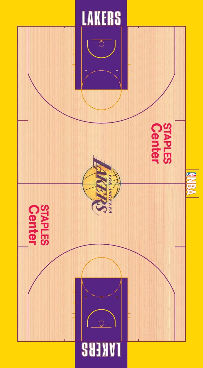
There is a lot of things can be done for exploratory analysis with this data set, and I’m really excited about it as a long-term Kobe fan. First let’s load the data up.
library(ggplot2)
library(data.table)
df <- read.csv('data.csv')
df <- setDT(df)
# exclude team_id, team_name, etc.
df[, team_id := NULL]
df[, game_id := NULL]
df[, game_event_id := NULL]
df[, team_name := NULL]
df[, shot_made_flag:= as.factor(shot_made_flag)]

# parse out home vs. away
df[matchup %like% "@", matchup := 'Away']
df[matchup %like% "vs.", matchup := 'Home']
df[, season_num := as.numeric(season)]

# set game_date into data format
df[, game_date:= as.Date(game_date)]

#split into train & test data
train <- df[!is.na(shot_made_flag), ]
test <- df[is.na(shot_made_flag), ]

# split into regular season and playoffs
regular <- train[playoffs == 0]
playoffs <- train[playoffs == 1]

# load basketball court
library(jpeg)
library(grid)
courtimg <- readJPEG('lakers.jpg')
courtimg <- rasterGrob(courtimg, width=unit(1,"npc"), height=unit(1,"npc"))
A function to plot kobe’s shots on the court, I’ve adjusted the image to line-up with the image, though it is still a little bit off.
# base plot function
plot_kobe <- function(data, cat, alpha = 1){
    p <- ggplot(data, aes(data[, loc_x], data[, loc_y], color = data[[cat]]))+
            annotation_custom(courtimg, -300, 300, -115, 900)+
            geom_point(alpha = alpha)+
            theme_bw()+
            ylim(-80, 400)+
            xlim(-280, 280)+
            xlab('X')+
            ylab('Y')+
            scale_color_manual('Shots', values = c('#e61919', '#009999'))
return(p)
}
Let’s first get an impression of all Kobe’s jump shots. He loved to shoot at 45 degrees on both sides of the court, beyond the 3-point line as well as in the middle range.
ggplot(train[action_type == 'Jump Shot'], aes(color = shot_made_flag)) +
        annotation_custom(courtimg, -300, 300, -115, 900)+
        stat_density2d(geom = 'polygon', contour = T, n = 500, aes(x = loc_x, y = loc_y,
                                                      fill = ..level.., alpha = ..level..))+
        theme_bw()+
        ylim(-80, 400)+
        xlim(-280, 280)+
        xlab('X')+
        ylab('Y')+
        scale_fill_gradient('Density', low = '#b3d1ff', high = '#003d99')+
        scale_color_manual('Shots', values = c('#ff0000', '#00ffcc'))+
        facet_wrap(~shot_made_flag)
So, how deadly is Black Mamba? Here is a plot of Kobe’s shots in the fourth quarter with less than 24 seconds left (last attack chance)
plot_kobe(train[minutes_remaining <= 1 & period == 4 & seconds_remaining <= 24],
                cat = 'shot_made_flag')
Then, what about his shooting percentage? Kobe is often scolded by his low shooting accuracy and bad shot selection. Here is the function to calculate his shooting performance. Note that type is default at 0 (all shot types selected). Type = 2 is to calculate two pointers, and 3 for three pointers.
shoot_percentage <- function(data, type = 0){
    if (type == 0){
    shots <- as.numeric(as.character(data[, shot_made_flag]))
    } else if (type == 2){
        shots <- as.numeric(as.character(data[shot_type == '2PT Field Goal'
                                              , shot_made_flag]))
    } else {
        shots <- as.numeric(as.character(data[shot_type == '3PT Field Goal'
                                              , shot_made_flag]))
    }
    percentage <- sum(shots)/length(shots)
return(percentage)
}
Kobe’s two points shooting percentage in last 24 seconds of a game:
shoot_percentage(train[minutes_remaining <= 1 & period == 4 & seconds_remaining <= 24], 2)## [1] 0.4752747# at home:
shoot_percentage(train[minutes_remaining <= 1 & period == 4 & seconds_remaining <= 24
& matchup == "Home"], 2)## [1] 0.4720497# Away
shoot_percentage(train[minutes_remaining <= 1 & period == 4 & seconds_remaining <= 24
& matchup == "Away"], 2)## [1] 0.4778325It seems that Kobe’s shooting performance (2 pointers) is the best during away games, let’s see his shooting locations:
plot_kobe(train[minutes_remaining <= 1
                & period == 4
                & seconds_remaining <= 24
                & shot_type == '2PT Field Goal'
                & matchup == "Away"], cat = 'shot_made_flag')
2. Now, let’s examine the Kobe’s regular season vs. playoffs performances
A function to calculate shooting percentage by continous scales and another function to plot the shooting percentages.
# calculate shooting percentage by factor
sp_fac <- function(data, factor){
    sp <- numeric()
    start <- range(data[[factor]])[1]
    end <- range(data[[factor]])[2]
    for(i in start:end){
        temp <- data[data[[factor]] == i]
        if (start != 1){
            diff <- start - 1
            sp[i - diff] <- shoot_percentage(temp)
        } else {
            sp[i] <- shoot_percentage(temp)
        }
    }
return(sp)
}

# plot shooting percentage by factor
plot_sp <- function(regular, playoffs, factor){
    len <- c(length(regular), length(playoffs))
    n <- max(len)
    if (len[1] > len[2]) {
        playoffs <- c(playoffs, rep(NA, len[1] - len[2]))
    } else {
        regular <- c(regular, rep(NA, len[2] - len[1]))
    }

    data <- data.frame(fac = c(1:n),
                       regular = regular,
                       playoffs = playoffs)

    p <- ggplot(data, aes(x = fac))+
            geom_line(aes(y = regular, color = 'regular season'), size = 1.2)+
            geom_line(aes(y = playoffs, color = 'playoffs'), size = 1.2)+
            ylab('shooting percentage')+
            ylim(c(0, .6))+
            xlab(factor)+
            scale_color_manual(name = 'Type', values = c('#e61919', '#00cc99'))+
            theme_bw()
return(p)
}
plot shooting percentage by distance
sp_reg_bydistance <- sp_fac(regular, 'shot_distance')
sp_po_bydistance <- sp_fac(playoffs, 'shot_distance')
plot_sp(sp_reg_bydistance, sp_po_bydistance, 'Distance')
plot shooting percentage by game period
sp_reg_byperiod <- sp_fac(regular, 'period')
sp_po_byperiod <- sp_fac(playoffs, 'period')
plot_sp(sp_reg_byperiod, sp_po_byperiod, 'period')
plot shooting percentage by season
sp_reg_byseason <- sp_fac(regular, 'season_num')
sp_po_byseason <- sp_fac(playoffs, 'season_num')
plot_sp(sp_reg_byseason, sp_po_byseason, 'Seasons')
plot shooting percentage in the 4th quarter
sp_reg_4th <- sp_fac(regular[period == 4, ], 'minutes_remaining')
sp_po_4th <- sp_fac(playoffs[period == 4, ], 'minutes_remaining')
plot_sp(sp_reg_4th, sp_po_4th, 'Minutes Remaining') +
    xlim(c(11, 0))