Canonical Vectors in R
WW44SS
April 8, 2016
SUMMARY
Word vectors rely on deep-learning based word-correlation analysis of texts with ~ billions of words to provide interesting linear structures in the word-vector space which convey relationships between words. This analysis explores some of the “canonical” examples of word vector relations - mostly as an exercise to see if I can reproduce known results before embarking on my own anlaysis.
An interesting finding is that while the scalar product of two vectors reveals the \(\cos\) difference between vectors, there appears to be more information in looking at the similarity of a spectrum of like words.
DATA SOURCES AND METHODS
The deep learning for word-vector analysis relies on the “pre-trained” GloVe vectors from Jeffrey Pennington, Richard Socher, and Christopher D. Manning. 2014.
WORD VECTOR ANALYSIS
The first step is to load the GloVe word vectors.
    number.of.words<-9900
    word.vector.file<-"glove.6B.300d.txt"
The analysis uses the first 9900 of the GloVe word vectors glove.6B.300d.txt. It took 24 seconds to process the data into a data frame.
WORD VECTOR SIMILARITY
Before delving into the full analysis, it’s helpful to look at vector representations of familiar word-pairs to help build an intuitive sense of how vector representations of words facilitate their coparison and analysis.
Vectors of individual words are easily extracted from the word vector data frame using simple regular expressions syntax.
Vector frepresenting the word man are computed from the functions
man.vec <- "man" %>% vectorize.word
man.vec.n <- "man" %>% vectorize.word.n
where \(\textbf{man.vec}\) and \(\textbf{man.vec.n}\) represent full length and unit vectors of the word “man”.
In addition, I made a function to look for words from a common stem. For instance
man.stem.vec.n <- "man" %>% vectorize.stem.ncreates a unit vector \(\textbf{man.stem.vec.n}\) representing the following 27 words: many, man, management, manager, managed, manufacturing, manchester, manhattan, managing, manufacturers, managers, manner, manage, mandate, manila, manufacturer, manuel, mandela, manages, manufactured, mansion, mandatory, manual, manning, manufacture, manor, and manuscript.
As illustrated here, this needs to be used with care, since several of the words have only peripheral assocation with the intended stem.
UNDERSTANDING WORD VECTORS
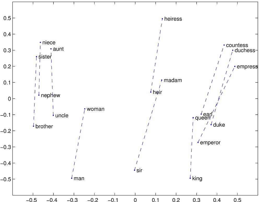
Let’s reproduce a well-known and intuitively appealing example of word vector comparisons. Looking at vectors of male-female relationship, we can see how the vectors develop.
The goal is to approximately reproduces results here ). The postion of each word represents the “vector” of that word (noting that this is a two dimenstional representation of a 300 element vector). Here vectors are not normalized.
WITH FULL LENGTH VECTORS

this produces unsatisfactory results. Specifically, vector alignment is not as expected.
WITH UNIT NORMALIZED VECTORS
Repeating the experiment with normalized vectors (set to unit length) gives a better result.

Recalling basic properties of vector addition, we can see (approximately):
\[ \begin{aligned} \textbf{pseudo.man} = \textbf{male} + \textbf{woman} - \textbf{female} \approx \textbf{man} \end{aligned} \]
\[ \begin{aligned} \textbf{pseudo.king} = \textbf{man} + \textbf{queen} - \textbf{woman} \approx \textbf{king} \end{aligned} \]
While these identities are not precisely satisfied in the two dimensional representation of the 300 element word vectors, we can quantify differences more precisely by taking the quantity
\[ \begin{aligned} \cos{\theta_{d}} = \| \textbf{pseudo.d} \cdot \textbf{d} \| / ( \| \textbf{d} \| \| \textbf{pseudo.d} \| )) \end{aligned} \]
where
\[ \begin{aligned} \textbf{pseudo.d} \equiv \textbf{a} + \textbf{b} - \textbf{c} \approx \textbf{d} \end{aligned} \]
In this case \(\cos{\theta_{king}}\) = 0.664 and the \(\cos{\theta_{man}}\) = 0.702. The question is, how good is this? These implied angles are on the order of 45 degrees. (while this may not seem very good based on intuition rooted in the unit circle, recall we are dealing with vectors in 300 dimensions.
HOW DO VECTORS THEMSELVES COMPARE?
To get an idea of the significance, let’s compare the similarity of the pseudo.vector to the word itself.
As a first stab, the plot below simply encodes the value of each vector component. While the vector for \(\textbf{king}\) and \(\textbf{pseudo.king}\) are similar, it’s hard, at least for for me, to distinguish the two have very much in common. For instance, \(\textbf{king}\) any closer to \(\textbf{woman}\) than to \(\textbf{man}\)? In retrospect this is not surprising. The vectors are highly abstracted representations that make sense only in the context of other words.
## Using names as id variables
WORD TO WORD COMPARISON IS MORE INTERESTING
It turns out it’s much more interesting to look at vectors in the context of actual words. The plots below I’ve taken the scalar product of the vectors \(\textbf{king}\) and \(\textbf{pseudo.king}\) with \(\textbf{king}\) and some neighboring words (for all intents, random).

This is just a sample of the nearest 88 neighboring words. Note that both the \(\textbf{king}\) and \(\textbf{pseudo.king}\) have a high scalar product with the vector representing \(\textbf{king}\), whereas the root vector \(\textbf{man}\) does not.
Another point is the relatively higher scalar products of the pseudo.vector with words like “britain” and “george” also stand out. This is important to recognize in relation to “compounded meaning” of text in relation to specific words.
As a comparison the plot below shows the scalar products for \(\textbf{king}\) and \(\textbf{man}\) with neighboring words. This reveals the scope of the change in the vector, and some sense the meaning of the word.
 The differences between vectors is plotted below.

A histogram of the differences show a fairly tight distribution.

Here is a comparison to the root vector \(\textbf{man}\)

Note this histogram is not as tight as above, representing larger differences to the target \(\textbf{king}\).

LETS LOOK AT CITY STATE PAIRS
This is a trial to test how capitol and state pairs line up. The poor comparison is diffult to because these words, for instance Reno tend to have context differences beyond the association implicit here. This ambiguity presents challenges in using vectors to interpret text meaning and bias, since these different contexts may confound specific interpretations.

COMPARING WITH OTHER WORDS
Let’s see how \(\textbf{texas}\) and \(\textbf{pseudo.texas}\) line up with neighboring words. In this case let’s test
\[ \begin{aligned} \textbf{pseudo.texas} \equiv \textbf{california} + \textbf{austin} - \textbf{sacramento} \approx \textbf{texas} \end{aligned} \]
Here is a graph comparing \(\textbf{pseudo.texas}\) and \(\textbf{texas}\).

It’s evident this does not substantially improve upon comparing \(\textbf{california}\) and \(\textbf{texas}\)

It’s hard to explain why this doesn’t work well without doing more work. But it appears that when the basis word (e.g. “california”) is reasonably close to the target word (e.g. “texas”) already this technique is less effectve without accounting for greater scope of differences between then. For instance, perhaps adding more city pairs (e.g. Los Angeles and Dallas, Houston and San Francisco) would improve the result?
OCCUPATIONS
This test shows professional words line up reasonably well. Not all tested samples worked as well (for instance “doctor” and “medicine” don’t fall in neatly) as these pairs did.

CONCLUSIONS
It’s straight forward to reproduce “canonical” examples of word vector relations. They seem to work as advertised in some, but not all, cases.
In some cases “intuitive” word pairs don’t necessarily follow the expected patterns.
While word vectors are a substantial advance in understanding like meaning of words, there are limitations which need to be comprehended in any application. Simply picking word pairs which seem to have common relationships does not automatically guarantee these are reproduced in a word vector analysis.