Various map types:

• Road maps
• Satellite maps
• Terrain maps/physical maps
• Abstracted maps

There are more which will be presented next week…

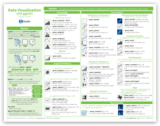
The R-package ggmap will be used in the following to produce different types of maps with the command qmap

Source

A road map is one of the most widely used map types.

• These maps show major and minor highways and roads (depending on detail)
• as well as things like airports, city locations and points of interest like parks, campgrounds and monuments.
• Major highways on a road map are generally red and larger than other roads,
• while minor roads are a lighter color and a narrower line.

• We'll need package ggmap - so we have to install it:

1. possibility

install.packages("ggmap")

1. possibility:

• To load the library we use the command library

library(ggmap)

qmap("Mannheim")

• level 3 - continent
• level 10 - city
• level 21 - building

qmap("Germany", zoom = 6)

?qmap

Different components in the help

• Description
• Usage
• Arguments
• Value
• Author(s)
• See Also
• Examples

Extract from the help file on qmap:

This examples can be directly copy-pasted to the console

qmap(location = "baylor university")
qmap(location = "baylor university", zoom = 14)
# and so on

qmap('Mannheim', zoom = 14, source="osm")

qmap('Mannheim', zoom = 14, source="osm",color="bw")

qmap('Mannheim', zoom = 14, maptype="satellite")

qmap('Mannheim', zoom = 21, maptype="hybrid")

Physical maps illustrate the physical features of an area, such as the mountains, rivers and lakes. Colors are used to show relief differences in land elevations.

• The water is usually shown in blue.
• a lighter color is typically used at lower elevation and
• darker color indicate higher elevations.
• Contour lines can also be used to show elevation changes (they are normally spaced at regular intervals)

qmap('Schriesheim', zoom = 14,
 maptype="terrain")

Source: Design faves

• Abstraction is used to create a map with only essential information
• Example metro maps - directions and little information for orientation is included
• In the following especially background maps

qmap('Mannheim', zoom = 14,
 maptype="watercolor",source="stamen")

qmap('Mannheim', zoom = 14,
 maptype="toner",source="stamen")

qmap('Mannheim', zoom = 14,
 maptype="toner-lite",source="stamen")

qmap('Mannheim', zoom = 14,
 maptype="toner-hybrid",source="stamen")

qmap('Mannheim', zoom = 14,
 maptype="terrain-lines",source="stamen")

These high-contrast B+W (black and white) maps are featured in our Dotspotting project. They are perfect for data mashups and exploring river meanders and coastal zones.

Source: http://maps.stamen.com/

• <- is an assignment operator which can be used to create an object
• This is useful if you work with several maps at the same time

MA_map <- qmap("Mannheim", 
               zoom = 14,
               maptype="toner",
               source="stamen")

Geocoding (…) uses a description of a location, most typically a postal address or place name, to find geographic coordinates from spatial reference data …

Wikipedia - Geocoding

library(ggmap)
geocode("Mannheim Wasserturm",source="google")

   lon      lat

1 8.473664 49.48483

Source

Reverse geocoding is the process of back (reverse) coding of a point location (latitude, longitude) to a readable address or place name. This permits the identification of nearby street addresses, places, and/or areal subdivisions such as neighbourhoods, county, state, or country.

Source: Wikipedia

revgeocode(c(48,8))

[1] "Qoriley Rd, Somalia"

mapdist("Q1, 4 Mannheim","B2, 1 Mannheim")

        from             to   m    km     miles seconds

1 Q1, 4 Mannheim B2, 1 Mannheim 746 0.746 0.4635644 211 minutes hours 1 3.516667 0.05861111

mapdist("Q1, 4 Mannheim","B2, 1 Mannheim",mode="walking")

        from             to   m    km     miles seconds

1 Q1, 4 Mannheim B2, 1 Mannheim 546 0.546 0.3392844 420 minutes hours 1 7 0.1166667

mapdist("Q1, 4 Mannheim","B2, 1 Mannheim",mode="bicycling")

        from             to   m    km    miles seconds

1 Q1, 4 Mannheim B2, 1 Mannheim 555 0.555 0.344877 215 minutes hours 1 3.583333 0.05972222

POI1 <- geocode("B2, 1 Mannheim",source="google")
POI2 <- geocode("Hbf Mannheim",source="google")
POI3 <- geocode("Wasserturm Mannheim",source="google")
ListPOI <-rbind(POI1,POI2,POI3)
POI1;POI2;POI3

   lon      lat

1 8.462844 49.48569 lon lat 1 8.469879 49.47972 lon lat 1 8.473664 49.48483

MA_map +
geom_point(aes(x = lon, y = lat),
data = ListPOI)

MA_map +
geom_point(aes(x = lon, y = lat),col="red",
data = ListPOI)

ListPOI$color <- c("A","B","C")
MA_map +
geom_point(aes(x = lon, y = lat,col=color),
data = ListPOI)

ListPOI$size <- c(10,20,30)
MA_map +
geom_point(aes(x = lon, y = lat,col=color,size=size),
data = ListPOI)

from <- "Mannheim Hbf"
to <- "Mannheim B2 , 1"
route_df <- route(from, to, structure = "route")

More information

qmap("Mannheim Hbf", zoom = 14) +
  geom_path(
    aes(x = lon, y = lat),  colour = "red", size = 1.5,
    data = route_df, lineend = "round"
  )

• Article by David Kahle and Hadley Wickham on the usage of ggmap.
• Grab a map
• Making Maps in R

More about adding points

• Usage of geom_point
• Question on stackoverflow

• Cheatsheet on data visualisation

ggmap: Spatial Visualization with ggplot2

by David Kahle and Hadley Wickham