The Hidden Costs of Prosperity: Income, Housing, and Commuting Across 800 U.S. Counties
By Haleluya Tesfamariam
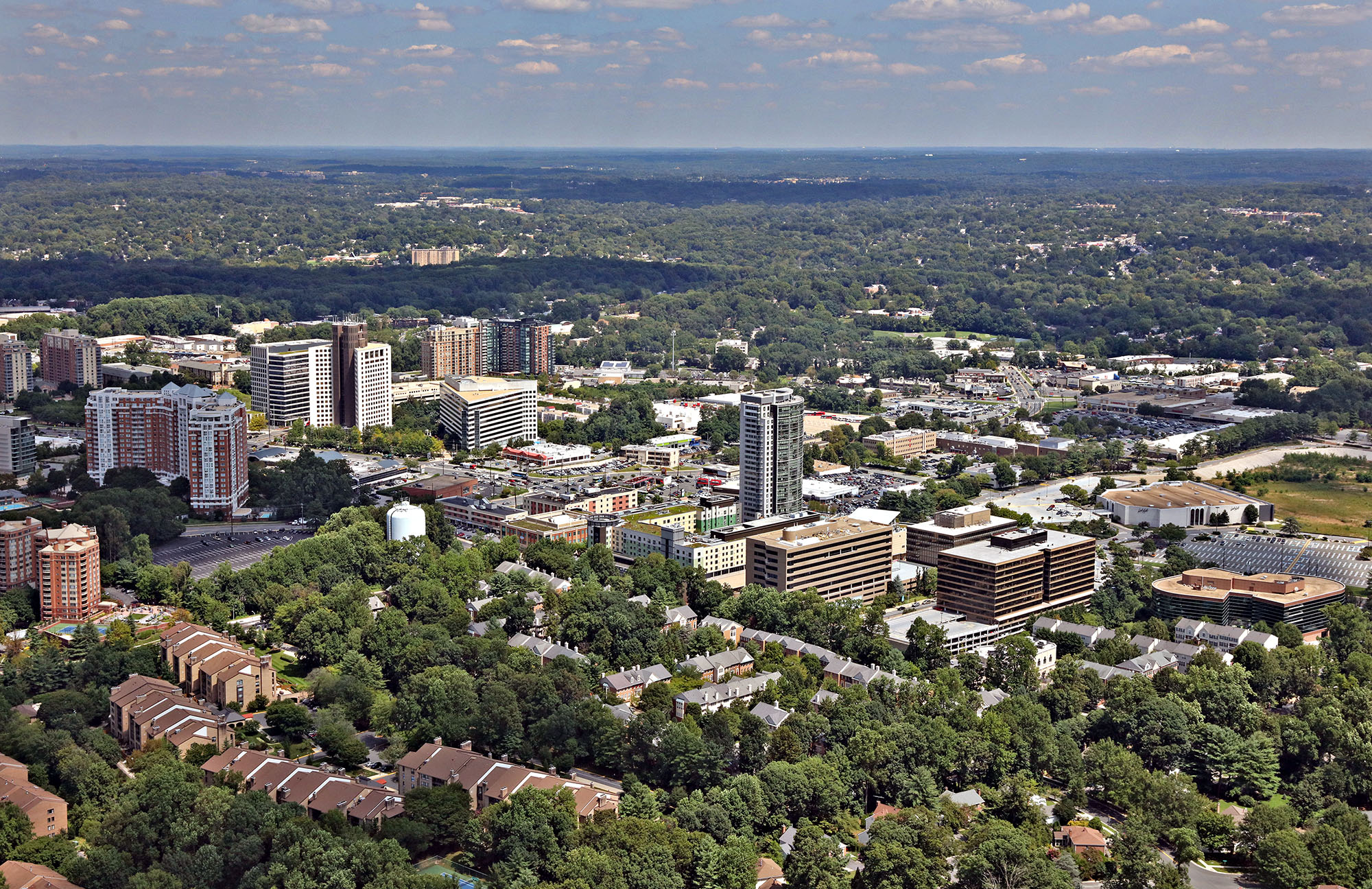
Aerial view of Rockville, Maryland, looking northeast, showing residential and commercial development. Photo by Duane Lempke, August 24, 2018.
Photo: Duane Lempke, August 24, 2018. Wikimedia Commons, CC0 1.0.
Introduction
Having lived in several parts of Montgomery County, Maryland, I have noticed that housing decisions involve more than the price of a home or apartment. Transportation, commuting time, and the cost of living also shape what a place is like for the people who live there.
This led me to a broader economic question: does greater prosperity necessarily translate into better living conditions? A county can have a high median household income while also facing expensive housing, long commutes, or crowded homes. Income alone may not show the full picture. In this project, I examine how income relates to three parts of county life: housing cost burden, commuting time, and residential crowding. I also look at poverty, unemployment, and regional differences to see whether these patterns are consistent across the country.
To investigate this question, I used the ACS 5-Year Socioeconomic Estimate Data by County, published by the U.S. Department of Housing and Urban Development (HUD) on Data.gov and based on the 2016-2020 American Community Survey (ACS) five-year estimates from the U.S. Census Bureau. The original file has 3,221 rows (one per county) and 146 columns. I kept 8 analysis variables: 6 quantitative variables (median household income, poverty rate, unemployment rate, average commute time, housing cost burden, and crowded housing) and 2 categorical variables (region and income tier). The two categorical variables were not in the original file; I created them with mutate().
To prepare the data, I used filter() to remove Washington, D.C. and Puerto Rico, leaving counties in the 50 states. I then used arrange() and head() to keep the 800 counties with the largest populations. I used mutate() to create the region and income tier categories, and select() to keep the variables used in the analysis and give them readable names. This focuses the project on the most populated counties, rather than trying to describe every county in the country.
Research question: Across the 800 most populated U.S. counties, does higher median household income correspond with lower housing cost burden, shorter commutes, and less residential crowding, and how do these relationships differ by region?
Variables/Schema
Quantitative:
income: median household income in the past 12 months, in thousands of dollars (original column B19013EST1, divided by 1,000).
poverty: percent of people living below the poverty line (B17021EST2_PCT).
unemployment: percent of the labor force that is unemployed (B23001_UE_PCT).
commute: average travel time to work, in minutes (B08013_AVG_TTW).
cost_burden: percent of households spending 30% or more of their income on housing (B25106_CB_PCT).
crowding: percent of households that are crowded, meaning more than one person per room (B25014_CROWD_PCT).
Categorical:
region: Northeast, Midwest, South, or West, built from the state name using R’s built-in state.region list. The dataset gives the state, and match() looks up the matching region.
income_tier: low (under $60,000), middle ($60,000 to $79,999), or high ($80,000 and up), built from median household income. The tier is stored in order from low to high. Cut-offs are according to the department of Housing and Urban Development’s national estimated family incomes for fiscal 2020 (the last year in the dataset).
The columns county and state (names used for labeling) and population (used only to pick the 800 largest counties) are kept in the data but are not counted as variables in the analysis.
Libraries
library(readr)library(tidyverse)
── Attaching core tidyverse packages ──────────────────────── tidyverse 2.0.0 ──
✔ dplyr     1.2.1     ✔ purrr     1.2.2
✔ forcats   1.0.1     ✔ stringr   1.6.0
✔ ggplot2   4.0.3     ✔ tibble    3.3.1
✔ lubridate 1.9.5     ✔ tidyr     1.3.2
── Conflicts ────────────────────────────────────────── tidyverse_conflicts() ──
✖ dplyr::filter() masks stats::filter()
✖ dplyr::lag()    masks stats::lag()
ℹ Use the conflicted package (<http://conflicted.r-lib.org/>) to force all conflicts to become errors
Registered S3 method overwritten by 'quantmod':
  method            from
  as.zoo.data.frame zoo
Highcharts (www.highcharts.com) is a Highsoft software product which is
not free for commercial and Governmental use
Rows: 3221 Columns: 146
── Column specification ────────────────────────────────────────────────────────
Delimiter: ","
chr   (5): GEOID, STATE, STATE_NAME, COUNTY, NAME
dbl (141): OBJECTID_1, B08013EST1, B08013_AVG_TTW, B08303EST1, B08303_30MINU...

ℹ Use `spec()` to retrieve the full column specification for this data.
ℹ Specify the column types or set `show_col_types = FALSE` to quiet this message.
dim(acs)
[1] 3221 146
counties <- acs %>%#dropping dc and puerto rico, I only want the 50 statesfilter(STATE_NAME !="District of Columbia", STATE_NAME !="Puerto Rico") %>%#sorting so the most populated counties are on toparrange(desc(B17021EST1)) %>%head(800)
#making the two categorical variablescounties2 <- counties %>%mutate(#region: matching each state to r's built in list of regionsregion =as.character(state.region[match(STATE_NAME, state.name)]),#income tier: low / middle / high based on median incomeincome_tier =case_when( B19013EST1 <60000~"low", #under 60k B19013EST1 <80000~"middle", #60k up to 80k B19013EST1 >=80000~"high"#80k and up ),#putting the tiers in order so plots go low, middle, highincome_tier =factor(income_tier, levels =c("low", "middle", "high")) )
#keeping only what I need and renaming the cryptic codescounties3 <- counties2 %>%select(state = STATE_NAME,county = NAME,population = B17021EST1,#income starts in dollars, I convert it to thousands right after this selectincome = B19013EST1,poverty = B17021EST2_PCT,unemployment = B23001_UE_PCT,commute = B08013_AVG_TTW,cost_burden = B25106_CB_PCT,crowding = B25014_CROWD_PCT, region, income_tier ) %>%mutate(income = income /1000)#checking the final size (should be 800 rows)dim(counties3)
[1] 800 11
Visual & Data Exploration
#bar chart of region: how many counties are in each region?ggplot(counties3, aes(x = region)) +geom_bar(fill ="green") +labs(title ="Number of Counties in Each Region",x ="region",y ="number of counties")
#histogram of income: how are incomes spread out?ggplot(counties3, aes(x = income)) +geom_histogram(bins =30, fill ="blue", color ="white") +labs(title ="Median Household Income Across the 800 Biggest Counties",x ="median household income ($1,000s)",y ="number of counties")
#checking how much housing cost burden varies across countiesggplot(counties3, aes(x = cost_burden)) +geom_histogram(bins =30, fill ="orange", color ="white") +labs(title ="Housing Cost Burden Across the 800 Biggest Counties",x ="households spending 30% or more of income on housing (%)",y ="number of counties") +theme_minimal()
The initial exploration shows that income and crowding are both right-skewed. Most counties have median household incomes between about $50,000 and $70,000, while a smaller number reach roughly $147,000. Most counties have around 2% crowded households, but a few are above 10%. The South makes up the largest share of the sample (346 of 800 counties), and the low-income tier contains the most counties (362 of 800). Before beginning the analysis, I wanted to get a better understanding of the data and identify any potential biases, limitations, or overrepresentations within my sample. In addition, the distribution of housing cost burden showed that the share of households struggling with housing costs varies across counties. I wanted to look more closely at this measure and see what other economic conditions might be associated with higher housing cost burdens.
Regression: What Is Associated With Cost Burden?
#predicting housing cost burden from the other five quantitative variablesregression <-lm(cost_burden ~ income + poverty + unemployment + commute + crowding,data = counties3)summary(regression)
Call:
lm(formula = cost_burden ~ income + poverty + unemployment +
    commute + crowding, data = counties3)

Residuals:
    Min      1Q  Median      3Q     Max
-30.776  -3.197  -0.375   3.153  16.446

Coefficients:
             Estimate Std. Error t value Pr(>|t|)
(Intercept)   4.87131    1.86210   2.616  0.00906 **
income        0.16233    0.01839   8.826  < 2e-16 ***
poverty       0.47181    0.07007   6.733 3.19e-11 ***
unemployment  0.71517    0.15518   4.609 4.72e-06 ***
commute       0.03594    0.04114   0.874  0.38256
crowding      0.70442    0.10011   7.036 4.26e-12 ***
---
Signif. codes:  0 '***' 0.001 '**' 0.01 '*' 0.05 '.' 0.1 ' ' 1

Residual standard error: 4.685 on 794 degrees of freedom
Multiple R-squared:  0.3037,    Adjusted R-squared:  0.2993
F-statistic: 69.26 on 5 and 794 DF,  p-value: < 2.2e-16
Why these variables: I chose housing cost burden as the outcome because I wanted to understand how it relates to income, poverty, unemployment, commute time, and crowding. Including all five variables lets me examine their individual relationships while accounting for the others.
What it means: Income, poverty, unemployment, and crowding all have significant positive relationships with housing cost burden (p-values below 0.001). Commute time is not statistically significant (p = 0.383). The adjusted R² is 0.2993, meaning the model explains about 30% of the variation in housing cost burden across counties.
One interesting finding is that income also has a positive relationship with housing cost burden. This suggests that higher-income counties are not necessarily free from housing affordability pressures. The regression examines overall relationships, while the visualizations explore how conditions differ across regions. These results show association, not causation.
Visualization 1: Crowding Across Regions and Income Tiers
#average crowding for each region + income tier combocrowding_summary <- counties3 %>%group_by(region, income_tier) %>%summarize(avg_crowding =mean(crowding), .groups ="drop")ggplot(crowding_summary, aes(x = region, y = avg_crowding, fill = income_tier)) +#bars side by side for each tier, with a thin outline so the light bars show upgeom_col(position ="dodge", color ="gray30") +#non-default colors, light to dark for low to high incomescale_fill_brewer(palette ="Oranges") +labs(title ="Higher-Income Counties Are Not Less Crowded: Region Matters More Than Income",x ="Region",y ="Average Crowded Households (%)",fill ="Income Tier",caption ="Source: HUD / U.S. Census Bureau, ACS 5-Year Estimates 2016-2020") +theme_minimal()
What it shows: Each bar represents the average county-level percentage of crowded households for one region and income tier. This visualization uses both categorical variables to compare the geography of crowding with county income groups. Across the 800 counties, the low-, middle-, and high-income tiers each average about 2.5% crowded households. The regional differences are larger: the West averages about 4.6%, the South about 2.5%, the Midwest about 1.6%, and the Northeast about 1.4%. Even high-income counties in the West average about 4.9% crowded households, compared with about 1.3% for low-income counties in the Northeast. Within each region, the differences between income tiers are relatively small. This suggests that regional patterns are important when comparing crowding, and that county income tier alone does not explain much of the variation. The bars are averages of county percentages, so each county contributes equally rather than being weighted by its population. I would be interested in separating renters from homeowners in a future version, since the dataset includes housing information that could support a more detailed comparison.
Visualization 2: Housing Cost Burden Across Regions and Income Tiers
#average housing cost burden for each region + income tier comboburden_summary <- counties3 %>%group_by(region, income_tier) %>%summarize(avg_burden =mean(cost_burden), .groups ="drop")ggplot(burden_summary, aes(x = region, y = avg_burden, fill = income_tier)) +#bars side by side for each tiergeom_col(position ="dodge") +#non-default colors, light to dark for low to highscale_fill_brewer(palette ="YlGnBu") +labs(title ="Housing Cost Burden by Region and Income Tier",x ="Region",y ="Average Housing Cost Burden (% of Households)",fill ="Income Tier",caption ="Source: HUD / U.S. Census Bureau, ACS 5-Year Estimates 2016-2020") +#a different non-default theme than the first plottheme_classic()
What it shows: Each bar represents the average county-level share of households spending 30% or more of their income on housing, split by region and income tier. The relationship differs across the country. In the Northeast, the average burden rises from about 25% in low-income counties to about 31% in high-income counties. The West shows a similar pattern, rising from about 31% to 34%. In the South, the average stays nearly flat (about 28% to 29%), while in the Midwest it falls as income tier rises (about 26% to 23%). The main point is not that higher income causes housing costs to rise. Rather, higher-income counties are not automatically places where housing is affordable. In the Northeast and West especially, the higher-income county groups also have higher average housing cost burdens. As with the previous chart, these are unweighted averages of county percentages.
Visualization 3: Income and Commute Time (Interactive)
#interactive plot: hover over a dot to see which county it ishchart(counties3, "scatter",#one color group per region, and name = the county so it shows on hoverhcaes(x = commute, y = income, group = region, name = county)) %>%#four colors, one for each regionhc_colors(brewer.pal(4, "Set2")) %>%hc_title(text ="Higher-Income Counties Tend to Have Longer Commutes") %>%hc_xAxis(title =list(text ="Average Commute to Work (Minutes)")) %>%hc_yAxis(title =list(text ="Median Household Income ($1,000s)")) %>%#the text that shows up when the mouse is on a dot, taken from notes + highcharter guidehc_tooltip(pointFormat ="{point.name}: {point.x} min commute, ${point.y}k income") %>%hc_caption(text ="Source: HUD / U.S. Census Bureau, ACS 5-Year Estimates 2016-2020")
What it shows: Each dot represents one county. Moving to the right indicates a longer average commute, while moving up indicates a higher median household income. Hovering over a dot shows the county, its commute time, and income. The relationship is positive, with a correlation of about +0.51. Average commute time also increases across income tiers, from about 23 minutes in low-income counties to 30 minutes in high-income counties. This suggests that higher-income counties do not necessarily offer shorter commutes. One possible explanation is that many high-income counties are part of large metropolitan areas, although this dataset cannot confirm why.
Local Example: Montgomery County, Maryland
#pulling out montgomery county, marylandcounties3 %>%filter(state =="Maryland", county =="Montgomery")
# A tibble: 1 × 11
  state    county     population income poverty unemployment commute cost_burden
  <chr>    <chr>           <dbl>  <dbl>   <dbl>        <dbl>   <dbl>       <dbl>
1 Maryland Montgomery    1038784   112.    6.59         4.64    34.4        31.7
# ℹ 3 more variables: crowding <dbl>, region <chr>, income_tier <fct>
Montgomery County, Maryland provides a local example of the difference between income and other living conditions. Its median household income is about $112,000, well above the median for the 800 counties in this sample (about $62,000). At the same time, its average commute is about 34 minutes, compared with about 24 minutes for the median county. Its housing cost burden is about 32%, compared with about 27%, and about 3.1% of its households are crowded, compared with about 1.9%. This does not mean Montgomery County is simply a worse place to live. It shows that a high median income can exist alongside longer commutes and higher housing cost burdens. Crowding also needs context because household size and multigenerational living can affect the measure. As a local example, Montgomery County reinforces the main point of the project: income by itself does not capture every dimension of living conditions.
Limitations & Considerations
Time period and sample: The data uses five-year ACS estimates from 2016–2020, so it may not reflect current conditions. It also includes only the 800 most populated counties, excluding Washington, D.C. and Puerto Rico. The South makes up the largest share of the sample (346 of 800), which influences the overall comparisons.
The cleaned dataset does not include school access, public transportation availability, job accessibility, or actual home prices and rent levels. Using the original dataset would allow us to paint complete picture of living conditions. Combined with other HUD data, the analysis could also be expanded by separating renters from homeowners and examining how these relationships differ by region. Ultimately, the limitations of this dataset only allow us to identify associations not causation.
Conclusion
The results suggest that higher county income does not automatically correspond with lower housing cost burdens, shorter commutes, or less residential crowding. In the sample of 800 most populated U.S. counties, higher-income counties tend to have longer average commutes. In the Northeast and West, the higher-income county groups also have higher average housing cost burdens. Crowding varies more clearly across regions than across income tiers, with the West showing substantially higher average crowding than the Northeast. The regression adds another piece to the picture: income, poverty, unemployment, and housing cost burden are statistically associated with crowding in the model, while commute time is not statistically significant after the other predictors are included. Even so, the model explains only about a third of the variation in crowding.
Montgomery County offers a familiar example of these trade-offs. Its median income is much higher than the sample median, but its housing cost burden and average commute are also higher. This does not prove that prosperity creates these conditions. It shows why income should not be treated as a complete measure of how easy or affordable daily life is in a place. A fuller picture requires looking at several measures together and paying attention to regional differences. If I extended this project, I would compare renters and homeowners separately, add school and transportation access data, and examine the patterns at a smaller geographic level than counties.
Sources
Dataset
U.S. Department of Housing and Urban Development, Office of Policy Development and Research. (2025). ACS 5YR socioeconomic estimate data by county [Data set]. Data.gov. https://catalog.data.gov/dataset/acs-5yr-socioeconomic-estimate-data-by-county
U.S. Census Bureau. (n.d.). American Community Survey (ACS). https://www.census.gov/programs-surveys/acs
Image
Lempke, D. (2018, August 24). Aerial view of Rockville, Maryland, looking northeast [Photograph]. Wikimedia Commons. https://commons.wikimedia.org/wiki/File:RockvilleMarylandNortheast.jpg
R packages
Kunst, J. (2022). highcharter: A wrapper for the ‘Highcharts’ library [R package]. https://jkunst.com/highcharter/ Notes: I used the guide on hc_toolpoint() to help create the interactive plot’s labels.
Class notes
Notes and Code from classes of 10/28 and 11/02 were used to create the highcharter graph.
Notes from class of Week 4 were used to write the following data cleaning functions: arrange(), match(), mutate()