Agroforestry Biomass Supply Chain Design

Economic assessment and optimisation of AFS-based bioeconomy networks

Thomas Kirschstein and Nico Tauchnitz

Fraunhofer IKTS

2026-06-11

Overview

1. Introduction
2. AFS Systems, Value Creation & Biomass Growth
3. MILP Model for AFS Supply Chain Design (AFS-SCD)
4. Case Study: Saxony-Anhalt
5. Conclusion & Outlook

Introduction

What is the Bioeconomy?

“The bioeconomy encompasses the production of renewable biological resources and their conversion into food, feed, bio-based products, and bioenergy.” — European Commission, 2012; updated strategy 2018

• 🌾 Biomass as the primary feedstock (agriculture, forestry, marine)
• 🔬 Biotechnology enabling valorisation at molecular level
• ♻️ Circular economy integration — substitution of fossil feedstocks

Indicator	Value
Gross value added	€ 2.7 trillion
Employment	17.1 million jobs
Share of EU GDP	~11–16 %
Share of EU employment	~8 %

Growth Potentials: market segments — size & growth

Segment	Market 2025	CAGR to 2030/34
Bio-based chemicals (global)	$ 110–120 bn	9.6 %
Bio-based polymers (production)	4.5 mio. t	11.0 %
Biorefineries (global)	$ 57–146 bn	7.8–9.6 %
Biofuels (global)	~$ 145 bn	5.8 %
Bioplastics (global)	$ 11.9 bn	8.1 %

📦 Bio-based polymers capacity target: 8.5 mio. t by 2030 Bio-PP: +94 % new capacity

🧪 Platform chemicals Succinic acid, lactic acid — CAGR 5.9 %; market $ 28 bn by 2035

💊 Biopharmaceuticals (DE) € 19.2 bn revenue (2023); 34.5 % market share — fastest-growing pharma sub-sector

Biobased plastics

Total wood production in Germany: \(\approx\) 27 mill. t dry wood (2024), of which \(\approx\) 4–5 mill. t is beech (Bundesamt, 2026). UPM Biochemicals (Leuna) demands \(\approx\) 10 % of German beech production for biochemical conversion (UPM Biochemicals, 2024).

Feedstocks – Trees in Agricultural Systems

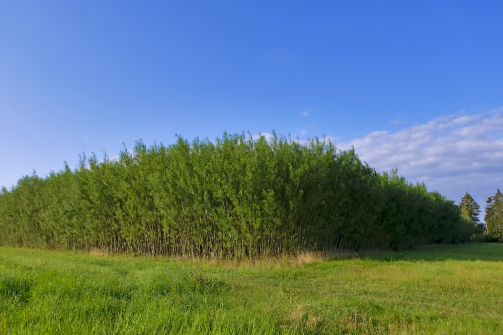
Short-Rotation Coppice (SRC)

• Monoculture, 8,000–20,000 trees/ha
• Rotation: 3–7 years; lifetime: 20–25 years
• No inter-row crop production

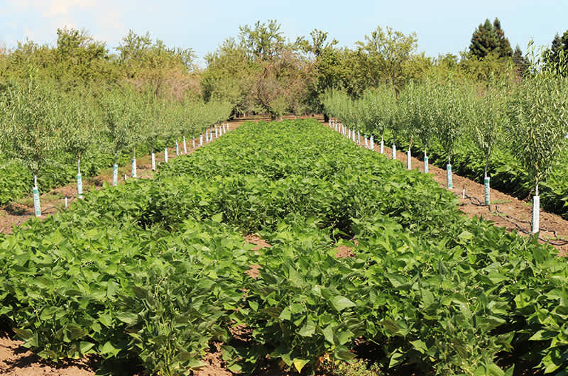
Agroforestry Systems (AFS)

• 1–4 tree rows in alley-cropping
• 10–30 % of total parcel area → 400–800 trees/ha
• Edge-tree effect

AFS Potential in Germany

• In Germany, ~1,200 ha of silvoarable AFS established in 2025 (≈ 0.02 % of agricultural land)
• Total agricultural land: ~17 mill. ha → potential AFS area: 1–2 mill. ha (6–12 %)
• Gross wood potential from AFS: 10–30 mill. t dry wood per year

Research question: How can AFS-based biomass supply chains be designed to make AFS economically attractive for farmers and industries?

AFS Systems, Value Creation & Biomass Growth

Economics of Agroforestry Systems

• Costs:
  • Establishment: 1,500–3,500 €/ha for planting, site prep (Faasch and Patenaude, 2012)
  • Maintenance: ~10 €/ha/yr (pruning, pest management)
  • Harvest: 200–400 €/ha (Testa Di Trapani et al., 2014)
  • Opportunity: foregone crop revenues (400–600 €/ha/yr in fertile regions)
• Returns:
  • Wood & biomass revenues
  • Crop yield premium in inter-row strips (+5–15 % relative to open-field) (Graves Burgess et al., 2007)
  • Subsidies and carbon credits (Toensmeier, 2017)

Profitability depends critically on which value chains absorb harvested biomass fractions.

Usage of AFS Biomasses

Biomass fractions

• 🪵 Stem wood
  Diameter: > 15 cm

• 🌿 Large branches
  Diameter: 7–15 cm

• 🍃 Small branches / leaves
  Diameter: < 7 cm

Cascade principle

Stem → Branch → Residue
High-value material uses should be prioritised before energetic use; residual fractions can then be routed to heat, power, or biogas pathways.

Application	Main products	Suitable fractions
🪑 Furniture industry	Sawn timber, veneers	Stem wood
📄 Paper industry	Pulp, fibres, cardboard	Stem + large branches
🧪 Chemical industry	Bioplastics, lignin derivatives, resins	Stem + large branches
🔥 Energy generation	Wood chips, pellets, CHP	All fractions
🫧 Biogas plant	Anaerobic digestion, electricity + heat	Leaves + fine brushwood

Modelling Biomass Growth – Gompertz Stand Model

Stand-level Gompertz model: \(M(t) = A \cdot e^{-e^{-k \cdot (t - t_0) }}\)

• \(A\) — asymptotic biomass quantity
  
• \(t_0 \in [9, 10]\) – inflection point maximal growth rate
  
• \(k \in [0.17, 0.2]\) – shape/skewness of growth curve

Compartment fractions (logistic model)

\(q_p(t) = \frac{f_p}{1 + \exp(-r_p \cdot (t - t_{50,p}))}\)

Calibrated for stem (\(d \geq 15\) cm) and branches (\(d \geq 7\) cm) residue defined as rest (Jha, 2018); (Civitarese Acampora et al., 2019)

MILP Model for AFS Supply Chain Design (AFS-SCD)

Model Structure and Decisions

Objective (AFS-SCD): Maximise total supply chain profit over a planning horizon of \(T\) years, integrating establishment, harvesting, logistics, and product cascading decisions.

Sets & variables:

• Stage 1: potential AFS sites \(\mathcal{I}\)
• Stage 2: Pre-treatment / storage nodes \(\mathcal{J}\)
• Stage 3: Industrial consumers \(\mathcal{K}\)
• \(z_{ist}\) — area of site \(i\) with AFS operated under arc \((s,t)\)
• \(X_{ijpt}\) / \(X_{jkpp't}\) — biomass transport from site \(i/j\) to \(j/k\)
• \(S_{jpt}\) — end-of-period inventory at facility \(j\)

Age-Lag Arc Structure for Harvest Scheduling

For planning horizon \(T=8\), \(A^{\min}=3\), \(A^{\max}=5\):

Example path: establishment in \(t=1\), harvests in \(t=5\) and \(t=8\)

Objective Function (AFS-SCD)

\[\begin{aligned} \max\; Z \;=\;& \sum_{k,\,p} R_{kp} \cdot\sum_{j,\,(p',p),\, t} X_{jkp'pt} &\text{Revenue} \\ &- \sum_{i} c^{\text{est}}_i \cdot\sum_{(0,t)\in\mathcal{S}^{est}} z_{i0t} &\text{Establishment cost}\\ &- \sum_{i} (c^{\text{main}}_i + c^{\text{opp}}_i) \cdot (t-s) \cdot \sum_{(s,t)\in\mathcal{S}^{harv}} z_{ist} &\text{Maintenance + Opportunity cost}\\ &- \sum_{i} c^{\text{harv}}_i \cdot \sum_{(s,t)\in\mathcal{S}^{harv}} z_{ist} &\text{Harvest cost}\\ &- \sum_{i,\,j,\,p,\,t} c^{\text{tr-raw}}_p \cdot d_{ij} \cdot X_{ijpt} &\text{Raw transport cost}\\ &- \sum_{j,\,k,\,(p,p'),\,t} c^{\text{tr-pre}}_{p'} \cdot d_{jk} \cdot X_{jkpp't} &\text{Pre-processed transport cost}\\ &- \sum_{j,\,p,\,t} c^{\text{stor}}_j \cdot S_{jpt} &\text{Storage cost} \end{aligned}\]

\(c^{\text{opp}}_i\) can be negative (subsidies / positive crop-yield spillovers) or positive (high-value arable land). Opportunity costs and transport costs are the two largest cost drivers (Faasch and Patenaude, 2012).]

Some constraints

Establishment per site: \[\sum_{(0,t)\in\mathcal{S}^{est}} z_{i0t} \leq \text{AREA}_i \qquad \forall\; i\]

Flow conservation (path connectivity): \[\sum_{(s,t)\in\mathcal{S}} z_{ist} = \sum_{(t,u)\in\mathcal{S}} z_{itu} \qquad \forall\; i,\; t\]

Age-dependent biomass yield: \[\sum_{j} X_{ijpt} \leq \sum_{(s,t)\in\mathcal{S}^{harv}} \eta_{p(t-s)} \cdot z_{ist} \qquad \forall\; i,p,t\]

where \(\eta_{pa} = q_p(a) \cdot M(a)\) links Gompertz stand model to logistics flows.

Quality cascade demand: \[\sum_{j,\,(p',p)\in\mathcal{Q}} X_{jkp'pt} \leq D^{\max}_{kpt} \qquad \forall\; k,p,t\]

Higher-quality fractions (stems) can substitute lower-quality demands, not vice versa.

Case Study: Saxony-Anhalt

Study Region & Supply Chain Configuration

• Region: Tri-state area of Saxony-Anhalt, northern Thuringia, northern Saxony (Germany)
• Highest density of registered SRC Feldblöcke in eastern Germany
• Road distances: 10–180 km between AFS sites and consumer locations
• OSRM routing for realistic transport cost estimates

Sites \(\mathcal{I}\)

• Registered SRC parcels from InVeKoS land-use register
• Spatially clustered via DBSCAN + Ward.D2 HAC (max radius 15 km)

Consumers \(\mathcal{K}\):

Grade	Consumers	Prices
1 Chemical	Mercer Stendal, UPM Leuna	80–120 €/t
2 Pulp	6 smaller facilities	55–75 €/t
3 Energy	Residual absorbers	30–40 €/t

Case Study Data Overview

Figure 1

Parameter	Value
Farms \(\vert\mathcal{I}\vert\)	145 (from 2239 parcels)
Hubs \(\vert\mathcal{J}\vert\)	11
Consumers \(\vert\mathcal{K}\vert\)	28
Planning horizon \(T\)	40 periods
Max rotation age \(A_{\max}\)	15 years
Min rotation age \(A_{\min}\)	3 years
Raw transport \(c^{tr\text{-}raw}\)	0.08 €/(t·km)
Pre-treated transport \(c^{tr\text{-}pre}\)	0.06 €/(t·km)
Establishment cost \(c^{est}\)	2,500 €/ha
Harvest cost \(c^{harv}\)	150 €/ha
Mean opportunity cost \(c^{opp}\)	166 €/ha/yr

Optimisation Results

Establishment Decisions & Product Mix

Figure 2

Summary statistics:

• Total profit: 2411 Mill. €
• Yearly Profit: 60.3 Mill. €
• Active super-sites: 60/145
• Biomass produced: 37 Mt
• Sites with \(C_{\text{opp}} > 150\) €/ha/yr are not selected

Product Flows by Biomass Fraction and End Use

Figure 3

Harvesting Cycle Distribution

Figure 4

Majority of harvests at ages 4–10 years (trade-off: yield growth vs. opportunity cost). Secondary peak at 12–15 years for sites near P1 consumers with low opportunity costs.

Biomass Volumes over Planning Horizon

Figure 5

Throughput rises as newly established sites reach minimum harvest age, then stabilises. Stem biomass (P1) dominates early periods when merchantable stem fraction is highest.

Profit breakdown

Figure 6

Site profitability

Figure 7

Site profitability & opportunity cost

Figure 8

Conclusion & Outlook

Summary & Key Findings

AFS-SCD MILP integrates

1. Gompertz-based age-dependent yield functions,

2. age-lag arc constraints for endogenous rotation scheduling, and

3. multi-product quality cascade for joint optimisation of AFS supply chains.

Results for Saxony-Anhalt base case:

• 60 out of 145 super-sites selected; concentrated in Elbe/Saale floodplains
• Total net profit: Mill. € over 40 periods
• Mean harvest cycle: 12.7 years
• Opportunity costs and transport are the dominant cost drivers

Thank You

Questions?

Thomas Kirschstein Fraunhofer IKTS thomas.kirschstein@ikts.fraunhofer.de

References

Bundesamt, S. (2026). Gesamteinschlag nach Holzartengruppen. Statistisches Bundesamt.

Civitarese, V., A. Acampora, et al. (2019). “Production of Wood Pellets from Poplar Trees Managed as Coppices with Different Harvesting Cycles”. In: Energies 12.15. Open access, p. 2973. DOI: 10.3390/en12152973.

Faasch, R. J. and G. Patenaude (2012). “The economics of short rotation coppice in Germany”. In: Biomass and Bioenergy 45, pp. 27-40. ISSN: 0961-9534. DOI: 10.1016/j.biombioe.2012.04.012.

Graves, A. R., P. J. Burgess, et al. (2007). “Development and application of bio-economic modelling to compare silvoarable, arable, and forestry systems in three European countries”. In: Ecological Engineering 29.4, pp. 434-449. ISSN: 0925-8574. DOI: 10.1016/j.ecoleng.2006.09.018.

Jha, K. K. (2018). “Biomass production and carbon balance in two hybrid poplar (euramericana) plantations raised with and without agriculture in southern France”. In: Journal of Forestry Research 29.6, pp. 1689-1701. ISSN: 1007-662X. DOI: 10.1007/s11676-017-0555-3.

Testa, R., A. M. Di Trapani, et al. (2014). “Economic evaluation of introduction of poplar as biomass crop in Italy”. In: Renewable and Sustainable Energy Reviews 38, pp. 498-506. ISSN: 1364-0321. DOI: 10.1016/j.rser.2014.07.007.

Toensmeier, E. (2017). “The Carbon Farming Solution: A Global Toolkit of Perennial Crops and Regenerative Agriculture Practices for Climate Change Mitigation and Food Security”. In: The Carbon Farming Solution. White River Junction, VT: Chelsea Green Publishing. ISBN: 978-1-60358-571-2.

UPM Biochemicals (2024). UPM Biochemicals Leuna: Bioraffinerie für Laubholz-Biomassekonversion. Unternehmenswebsite. Abgerufen: April 2026. URL: https://www.upmbiochemicals.com/de/.