08/09, 2025

Goal & Overview

Objective: Build a distance‑weighted influence surface that reflects how much natural habitat area surrounds each pixel, combining:

  • Additive natural area within a 1000 m circular window (unique polygon areas in hectares; no double‑counting within a patch).
  • Inverse log distance decay from the nearest natural area.
Concept & Notation

A focal (1000 m radius) additive area surface based on unique polygons:

\[\textbf{LogArea} = \log\!\left(1 + \sum_{i \in W} A_i\right), \qquad A_i = \text{area (ha) of polygon } i.\]

  • Not a smoothing or mean; it is an additive mass of nearby natural area.
  • The influence surface then adds an inverse log distance term:

\[\textbf{InvLogDistance} = \frac{1}{1+\log(1+d)}.\]

Finally, we combine and (optionally) smooth:

\[\textbf{WeightedInfluence} = \text{LogAreaNorm} + \text{InvLogDistance}. \]

Pipeline at a Glance

  1. Build LogAreaRaw1000.tif (unique polygon areas within 1000 m).
  2. Transform to LogArea and normalize to LogAreaNorm.
  3. Compute Distance, then InvLogDistance (and optional smoothed version).
  4. Sum and normalize to create IDW/IDWSmoothed.
  5. Visualize focal region and overlays with polygons.

Step 0 — Inputs & CRS

# Example inputs
# - NatureNoLakes.tif : binary (1 = nature, 0 / NA otherwise)
# - AllPolygons.shp   : polygons of natural areas (for overlay display)
# - Denmark GADM      : country mask

NatureNoLakes <- terra::rast("NatureNoLakes.tif")
DK <- geodata::gadm("Denmark", level = 0, path = getwd()) |>
  terra::project(terra::crs(NatureNoLakes))

# Ensure expected projected CRS in meters
crs(NatureNoLakes)

Step 1 — Build LogAreaRaw1000.tif

Summary of computation (performed once, heavy I/O):

  1. Disaggregate multipart polygons.
  2. Compute polygon area in hectares.
  3. Rasterize area value to the grid.
  4. Apply 1000 m circular window with a custom unique‑sum focal function (avoid double‑counting within a patch).
  5. Mosaic tiles if needed and write COG.

Note: The focal step must sum unique values within the window so a single patch contributes its area only once per window, regardless of how many pixels it spans.

Step 1b — Log transform & normalize

LogAreaRaw <- terra::rast("LogAreaRaw1000.tif")
LogArea     <- log1p(LogAreaRaw)
SpatioTemporalCont::write_cog(LogArea, "LogArea.tif")

# Normalize to [0,1] for additive combination later
rng <- terra::minmax(LogArea)
LogAreaNorm <- LogArea / (rng[2])
SpatioTemporalCont::write_cog(LogAreaNorm, "LogAreaNorm.tif")

Visualizing Additive Area (1000 m window)

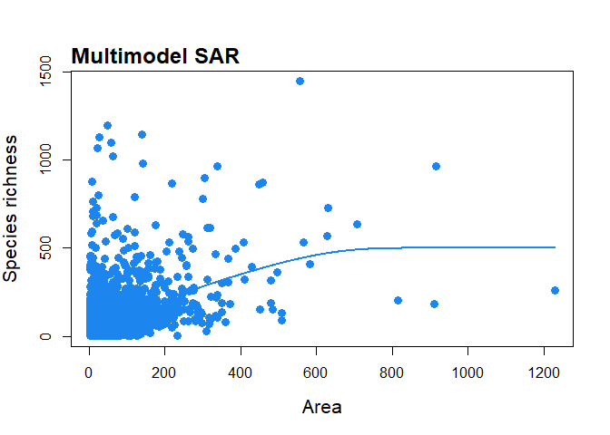
Area does not influence linearly

  • SAR

Visualizing LogArea (and normalized)

Step 2 — Distance to nearest natural area

Step 2b — Inverse log distance (and smooth)

$$ \[ \text{LogDistance} = \log(1+d)\] \[ \text{InvLogDistance} = \frac{1}{1+\log(1+d)}\] \[ \text{InvLogDistance}_{\alpha} = \left(\frac{1}{1+\log(1+d)}\right)^{\alpha} \quad (\alpha = 0.25)\]

$$

Visualization distances

Step 3 — Combine Area & Distance

\[\color{Purple}{\text{WeightedInfluence}} = \color{Red}{\text{LogAreaNorm}} + \color{Blue}{\text{InvLogDistance}}\]

Comparison with geotopes

Practical Notes & Caveats

  • Unique‑sum focal is essential to avoid over‑counting large polygons.
  • Choose the window radius (1000 m here) to match ecological processes/scales.
  • Normalize components before addition to keep each term in a comparable range.
  • Prefer COG outputs for large rasters; tile & mosaic when needed.
  • Consider sensitivity analysis: radius, decay exponent (e.g., 0.25), and alternative distance metrics.